Machine Learning Tutorial Python - 4: Gradient Descent and Cost Function

Summary

This script offers an insightful walkthrough of key machine learning concepts, focusing on the Mean Square Error (MSE) cost function, gradient descent, and the significance of the learning rate. The tutorial aims to demystify the mathematical underpinnings often encountered in machine learning, emphasizing a step-by-step approach to grasp these concepts without being overwhelmed. By the end, viewers are guided to implement a Python program that employs gradient descent to find the best fit line for a given dataset, illustrating the process through visual representations and debugging techniques. The practical exercise involves analyzing the correlation between math and computer science scores of students, applying the gradient descent algorithm to determine the optimal values of m and b, and ceasing iterations once a predefined cost threshold is met, showcasing the algorithm's convergence to the global minimum.

Takeaways

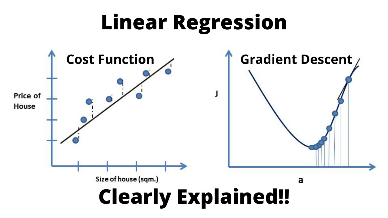
• 📘 Mean Square Error (MSE) is a popular cost function used in machine learning to measure the average squared difference between the estimated values and the actual value.
• 🔍 Gradient descent is an optimization algorithm used to find the best fit line by iteratively adjusting the parameters (m and b) to minimize the cost function.
• 📈 The learning rate is a key parameter in gradient descent that determines the size of the steps taken towards the minimum of the cost function.
• 📉 MSE is calculated as the sum of the squares of the differences between the predicted and actual data points, divided by the number of data points.
• 📊 To implement gradient descent, one must calculate partial derivatives of the cost function with respect to each parameter, which indicate the direction of the steepest increase.
• 🔢 The slope of the tangent at a point on a curve represents the derivative at that point, which is used to guide the direction of the step in gradient descent.
• 🔄 The process of gradient descent involves starting with initial guesses for m and b, then iteratively updating these values based on the partial derivatives and learning rate.
• 🔧 Numpy arrays are preferred for this type of computation due to their efficiency in matrix operations and faster computation speed compared to regular Python lists.
• 🔭 Visualization of the gradient descent process can be helpful in understanding how the algorithm moves through parameter space to find the minimum of the cost function.
• 🔴 The algorithm stops when the cost no longer decreases significantly, indicating that the global minimum has been reached or is very close.
• 🔬 Calculus is essential for understanding how to calculate the derivatives and partial derivatives that are used to guide the steps in gradient descent.

Q & A

What is the primary goal of using a mean square error cost function in machine learning?

The primary goal of using a mean square error cost function is to determine the best fit line for a given dataset by minimizing the average of the squares of the errors or deviations between the predicted and actual data points.

How does gradient descent help in finding the best fit line?

Gradient descent is an optimization algorithm that iteratively adjusts the parameters (m and b in the linear equation y = mx + b) to minimize the cost function. It does this by calculating the gradient (partial derivatives) of the cost function with respect to each parameter and updating the parameters in the direction that reduces the cost.

Why is it necessary to square the errors in the calculation of the mean square error?

Squaring the errors ensures that all errors are positive and prevents them from canceling each other out when summed. This makes it easier to optimize and find the minimum value of the cost function.

What is the role of the learning rate in the gradient descent algorithm?

The learning rate determines the size of the steps taken during each iteration of the gradient descent algorithm. It is a crucial parameter that affects the convergence of the algorithm; a learning rate that is too high may overshoot the minimum, while a rate that is too low may result in slow convergence or getting stuck in a local minimum.

How does the number of iterations affect the performance of the gradient descent algorithm?

The number of iterations determines how many times the gradient descent algorithm will update the parameters. More iterations allow for more refinement and potentially a better fit, but they also increase the computational cost. There is a trade-off between accuracy and efficiency that needs to be considered.

What is the significance of visualizing the cost function and the path taken by gradient descent?

Visualizing the cost function and the path of gradient descent helps in understanding how the algorithm navigates through the parameter space to find the minimum of the cost function. It provides insights into the convergence behavior and can help in diagnosing issues such as getting stuck in local minima or failing to converge.

Why is it important to start with an initial guess for m and b in the gradient descent algorithm?

Starting with an initial guess for the parameters m and b is important because gradient descent is sensitive to the starting point. Different starting points may lead to different local minima. However, with a well-behaved cost function, gradient descent can find the global minimum if the learning rate is properly chosen.

What are partial derivatives and how do they relate to the gradient descent algorithm?

Partial derivatives are derivatives of a function with respect to a single variable, keeping all other variables constant. In the context of gradient descent, partial derivatives of the cost function with respect to each parameter (m and b) provide the direction and magnitude of the steepest descent, which is used to update the parameters and 'descend' towards the minimum.

How can one determine when to stop the gradient descent algorithm?

The algorithm can be stopped when the change in the cost function between iterations falls below a certain threshold, indicating that the parameters have converged to a minimum. Alternatively, one can compare the cost between different iterations and stop when the cost does not significantly decrease, suggesting that further iterations will not yield a better fit.

What is the purpose of using numpy arrays over simple Python lists when implementing gradient descent in Python?

Numpy arrays are preferred over simple Python lists for their efficiency in performing matrix operations, which are common in gradient descent calculations. Numpy arrays are also faster due to their optimized implementations and support for vectorized operations.

In the context of the tutorial, what is the exercise problem that the audience is asked to solve?

The exercise problem involves finding the correlation between math scores and computer science scores of students using the gradient descent algorithm. The audience is asked to apply the algorithm to determine the best fit line (values of m and b) and to stop the algorithm when the cost between iterations is within a certain threshold.

Outlines

00:00

📚 Introduction to Machine Learning Concepts

The video begins by introducing key concepts in machine learning, such as the mean square error cost function, gradient descent, and learning rate. The speaker aims to demystify the mathematical equations often encountered in machine learning tutorials, encouraging viewers not to be intimidated by their math skills. The tutorial's goal is to implement gradient descent in a Python program, not just to solve a machine learning problem, but to understand the underlying processes for better use of libraries like sklearn. The importance of deriving a prediction function from a dataset is emphasized, using the example of predicting home prices based on area.

05:01

📈 Gradient Descent and Its Visualization

The second paragraph delves into how gradient descent operates, a method for finding the best fit line with fewer iterations. A visual representation is provided, plotting m (slope) and b (intercept) against the mean square error to form a 3D surface. Starting from an initial guess, the process involves taking small steps towards the minimum error, adjusting m and b iteratively. The concept of a learning rate is introduced, which, combined with the slope (or derivative), dictates the size of each step towards the optimal values of m and b.

10:02

🔢 Calculus and Derivatives in Gradient Descent

The third paragraph explains the role of calculus in determining the steps in gradient descent, focusing on derivatives as a means to calculate slopes. The basic concept of a derivative is introduced, including how to calculate it for a function at a particular point. The distinction between a regular derivative and a partial derivative is made, with examples provided. The video also references the channel '3Blue1Brown' for a more in-depth understanding of these mathematical concepts. Finally, the partial derivatives for m and b in the context of the mean square error function are derived and simplified for practical use in the algorithm.

15:05

💻 Implementing Gradient Descent in Python

The fourth paragraph outlines the practical implementation of gradient descent using Python. It begins with initializing m and b, defining the number of iterations, and setting up a loop to perform the iterative process. The loop calculates the predicted y values, the derivatives for m and b, and then updates m and b based on these derivatives and a learning rate. The learning rate is introduced as a key parameter that needs to be fine-tuned. The video also emphasizes the importance of tracking the cost at each iteration to ensure the algorithm is converging towards the correct solution.

20:06

🔍 Tuning the Learning Rate and Iterations

The fifth paragraph discusses the fine-tuning of the learning rate and the number of iterations for the gradient descent algorithm. It highlights the importance of monitoring the cost at each iteration to ensure it's decreasing, indicating that the algorithm is making progress. The speaker shares their approach to adjusting the learning rate, starting with a smaller value and increasing it to see the effect on cost reduction. The paragraph also demonstrates how an inappropriately large learning rate can cause the algorithm to overshoot the minimum and start increasing the cost. The goal is to find a balance where the cost continues to decrease with each iteration.

25:07

📉 Stopping Criteria and Application Exercise

The final paragraph introduces the stopping criteria for the gradient descent algorithm, which involves comparing the cost between iterations to a predefined threshold. The video uses a tolerance level to determine when the algorithm has converged sufficiently. It also presents an exercise for the viewer, which involves applying the gradient descent algorithm to find the correlation between math and computer science scores of students. The exercise aims to give practical experience in implementing and adjusting the gradient descent algorithm to achieve the best fit line for the given dataset.

Keywords

💡Mean Square Error (MSE)

Mean Square Error (MSE) is a measure of the average squared difference between the estimated values and the actual value. It is used as a cost function to quantify the performance of a predictive model. In the video, MSE is central to understanding how to evaluate the accuracy of the best fit line in a machine learning context. The script mentions that MSE is calculated by taking the sum of the squares of the differences between predicted and actual data points, then dividing by the number of data points.

💡Gradient Descent

Gradient Descent is an optimization algorithm used to minimize the cost function in machine learning models. It iteratively adjusts the parameters (like m and b in a linear model) to find the best fit line. The video explains that gradient descent allows for efficient finding of the best fit line with fewer iterations by taking 'baby steps' towards the minimum error, visualized as a descent towards the lowest point on a cost function surface.

💡Learning Rate

The learning rate is a parameter used in gradient descent to control the step size during the update of the model's parameters. It's crucial for the algorithm's convergence; a too-large rate may overshoot the minimum, while a too-small rate may lead to a very slow convergence. In the script, the learning rate is adjusted through trial and error to ensure that the cost is being reduced with each iteration, indicating that the algorithm is converging to the optimal solution.

💡Linear Regression

Linear Regression is a statistical method for modeling the relationship between a dependent variable 'y' and one or more independent variables denoted as 'x'. The video discusses linear regression in the context of predicting home prices using the area as the independent variable. The goal is to derive a linear equation that can predict future values based on past observations.

💡Cost Function

A cost function is a mathematical function that calculates the error of a model during training in machine learning. The mean square error is a common example of a cost function. The video emphasizes that the cost function evaluates how well the model's predictions match the actual data, and the goal of gradient descent is to minimize this cost.

💡Partial Derivative

A partial derivative is a derivative of a function with respect to one variable while keeping the other variables constant. In the context of the video, partial derivatives are used to calculate the slope of the cost function with respect to the parameters 'm' (slope of the line) and 'b' (intercept). These derivatives guide the direction of the 'baby steps' taken by the gradient descent algorithm.

💡Intercept (b)

In the context of a linear equation 'y = mx + b', the intercept 'b' is the point where the line crosses the y-axis. The video script discusses how 'b' is one of the parameters that need to be determined to find the best fit line using gradient descent, starting with an initial guess and iteratively adjusting it.

💡Slope (m)

The slope 'm' in a linear equation 'y = mx + b' indicates the steepness of the line and the direction of the increase or decrease in 'y' with respect to 'x'. The script explains that 'm' is another parameter to be found using gradient descent, which represents how much 'y' changes for a one-unit change in 'x'.

💡Training Data Set

A training data set is a collection of observations or data used for training a machine learning model. The video mentions that the training data set includes input-output pairs that the model uses to learn and derive the prediction function. It's the basis for calculating the error and subsequently the mean square error.

💡Python Programming

Python is a high-level programming language widely used in machine learning for its simplicity and the powerful libraries it offers, such as NumPy and scikit-learn. The video script includes a Python program that implements gradient descent to find the best fit line, demonstrating how theoretical concepts are applied in practice.

💡Jupyter Notebook

Jupyter Notebook is an open-source web application that allows creation and sharing of documents containing live code, equations, visualizations, and narrative text. The video script refers to using a Jupyter Notebook for visualization purposes, indicating its utility in machine learning for plotting data and observing the model's convergence.

Highlights

Mean square error cost function, gradient descent, and learning rate are fundamental concepts in machine learning.

The tutorial aims to demystify mathematical equations in machine learning and build a Python program for gradient descent.

Machine learning involves creating a prediction function from a dataset, unlike traditional linear algebra where equations are given.

The best fit line is derived from the dataset, representing the optimal equation for predicting future values.

Mean square error (MSE) is calculated by summing squared differences between actual and predicted data points, then dividing by the number of data points.

Gradient descent is an efficient algorithm for finding the best fit line with fewer iterations.

A visualization of the gradient descent process is provided to understand how m and b values are iteratively adjusted to minimize error.

The learning rate is a critical parameter in gradient descent, determining the step size towards the minimum error.

Derivatives and partial derivatives are essential for calculating the slope of the cost function at a given point.

The partial derivatives of m and b with respect to the cost function guide the direction of the next step in gradient descent.

Python code is used to implement gradient descent, using numpy arrays for efficient matrix operations.

The number of iterations and the learning rate are parameters that need to be fine-tuned for optimal performance.

Monitoring the cost at each iteration is crucial to ensure the algorithm is converging towards the global minimum.

The learning rate should be adjusted to ensure the cost is consistently decreasing, avoiding overshooting the minimum.

Gradient descent can be stopped when the cost between iterations falls below a certain threshold, indicating convergence.

A practical exercise is provided to apply the gradient descent algorithm to find the correlation between math and computer science scores.

The exercise involves using the gradient descent algorithm to determine the best fit line for predicting computer science scores from math scores.

The tutorial concludes with a discussion on stopping criteria for the gradient descent algorithm based on cost convergence.

Transcripts

mean square error cost function gradient

descent and learning rate

these are some of the important concepts

in machine learning

and that's what we are going to cover

today at the end of this tutorial we

would have written a python program

to implement gradient descent now when

you start going through machine learning

tutorials

the thing that you inevitably come

across is mathematical equations

and by looking at them the first thought

that jumps into your mind is oh my god i

suck at math i used to get 4 out of 50

in my math test

how am i going to deal with this let's

not worry too much about it

we can take one step at a time and the

things won't seem that much hard

also you won't be implementing gradient

descent

when solving the actual machine learning

problem

but the reason we are doing this

exercise today is that

you should know some of the internals so

that while using the sklearn library

you know what's going on and you can use

the libraries in a better way

with that let's get started during our

linear algebra class

in our school days what we used to have

was this equation

and x as an input and we used to compute

the value of y where the way you derive

9 is by multiplying this 3 with 2

which will be 6 plus 3 and that's how

you come up with 9.

in case of machine learning however you

have observations or training data set

which is your input and output

using that you try to derive an equation

also known as prediction function so

that you can use this equation

to predict uh future values of

x in case of

our problem of predicting home prices

we saw in the initial linear regression

tutorials that

we have area and price and using that we

came up with this equation now if you

don't know

this equation quite well you look at my

jupiter notebook

and in that notebook you'll see that i

have

this coefficient and intercept okay

so that's what i have put it here

so here i have the home prices in monroe

township

and i have plotted these on this chart

and what we are going to look at is

how can you derive this equation

given this input and output okay so

our goal is to derive this equation that

equation is nothing but

this blue line which is the best fit

line

uh going through all these data points

right now these data points are

scattered so it's not possible to draw

the perfect line but you try to draw a

line which which is

kind of a best fit all right but

the problem here is you might have

so many lines right that can pos

potentially go through these data points

my data set is very simple here if you

have

uh like very heavy data set and if it's

it's like scattered all over the place

then drawing these lines

becomes even more difficult so how do

you know

which of these lines is the best fit

line

okay so that's the problem that we are

going to solve today

so one way is you draw any random line

then from your actual data point

you calculate the error

between that data point and the data

point predicted by your line

okay so call it a delta you collect all

these deltas

and square them the reason you want to

square them

is these deltas could be negative also

and if you don't square them and just

add them then the results might be

skewed

after that you sum them up and divide it

by

n so n here is five it is number of data

points that you have available

the result is called mean square error

okay and mean square error is nothing

but

your actual data point minus the

predicted data point

you square it sum them up and then

divide by

n this mean square error

is also called a cost function there are

different type of cost function as well

but

mean square error is the most popular

one

and here y predicted is replaced by mx

plus b because you know that y is equal

to mx plus b

so that's the equation for mean square

error

now we initially saw that there are so

many different lines that you can draw

you're not going to try every

permutation and combination of

m and b because that is very inefficient

you want to take some efficient approach

where in very

less iteration you can reach your answer

okay and gradient descent is that

algorithm that helps you

find the best fit line in

very less number of iteration or in a

very efficient way

okay so we are going to look at how

gradient descent works now

for that i have plotted m b

against the mean square error or a cost

function

uh so here i have drawn different values

of

m and here there are different values of

p

which is your intercept and for

every value of m and b you will find

some cost so if you

keep on plotting those points here and

if you create a

plane out of it it will look like this

it will be like a ball

and what you want to do is you want to

start with

some value of m and b people usually

start with zero so here you can see

this point has m is zero and b is zero

and from that point you calculate the

cost so let's say the cost is

thousand then you reduce the value

of m and b by some amount and we'll see

what that amount is later on so you take

kind of like a mini step

you come here and you will see that the

error is now reduced to

somewhere around 900 something like that

and then again you reduce it by taking

one more step you keep on taking these

steps

until you reach this point which is

your minima here

the error is minimum and once you reach

that you have found your answer

because you will use that m and b

uh in your prediction function

i have plotted these different lines and

these different lines will have

different values of m and b

let's say this orange has m1 b1 so that

m1 b1 will be here somewhere

blue line will have m2 b2 m2 b2 will be

this red dot

then red line will have m3 b3 so m3 b3

will be somewhere here on this plot so

you can have like so many numerous lines

which can create this uh plot

now we just said that you will take this

baby step but how exactly you do it

because visually it sounds easy but

mathematically

when you give this task to your computer

uh

you have to come up with some concrete

approach all right

so we'll look into that but

here is the nice visualization of uh

how you can reduce your m and b

and reach the best fit line okay all

right

so let's look at how you're going to

take those baby steps

so i have these two charts uh if you

look at this 3d

plot from this direction what you will

see is a chart of

b against cost and that will be

this curvature similarly if you look at

this chart

from this direction the chart will look

something like this

and in both the cases you are starting

at this point which is this star

and then taking these many steps

and trying to reach this minimum point

which is this red dot

now how do you take these steps

right so one approach is let's say you

take

fixed size steps so here if you plot

this

against b i'm taking fixed size steps on

b

but the problem that it can create is by

taking these steps i

might miss the global minima okay i

might just miss it

and my gradient descent will never

converge it

from this point it will just start going

up and up and i don't know

where is my minima all right so this

approach is not going to work

what can work is if you take steps like

this

so here in each step i am following the

curvature

of my chart and also as i

reach near to my red point you can see

that

the step size is reducing you see like

this arrow is bigger and these arrows

are getting smaller and smaller

if i do something like this then

i can reach this minima now how do i do

that

so at each point you need to calculate

the slope

okay so for example at this point the

slope will be this this is a tangent

at the curvature and at this point here

my slope will be this

once i have a slope i know which

direction i need to go in for example

if you look at this green line and if

i'm at this blue dot

i know that i need to go in this

direction

and then there is something called a

learning rate which you can use

in conjunction with this slope here

to take that step and reach the next

point

now we have to get into calculus a

little bit

because calculus allows you to

figure out these baby steps and

when we are talking about these slopes

really this slope is nothing but a

derivative of

b with respect to this cost function

okay if you want to go in details i

recommend this channel three blue

one brown this guy is very good in

explaining mathematical concept

using a nice visualization so you will

really find it very useful

and pleasing but if you don't want to go

in details then

in this tutorial i'll just quickly walk

over some of the basic concepts okay

let's look at what is derivative so

derivatives is

all about slope i'm on this uh

website called math is fun and these

guys have explained it really well

so slope is nothing but a change in y

divided by change in x

okay so if you have line like this and

if you want to calculate slope between

the two points here

it is 24 divided by 15 but what if you

want to calculate the slope

at a particular point right like in our

case if you remember

here we want to calculate a slope at a

particular point

same thing here right so that slope

will be nothing but a small change in y

divided by small

change in x all right

we'll say as

x shrinks to 0 and y shrinks to 0

that's when you get more accurate slope

okay so for the equation like x square

that slope will be 2x okay

this is again called a derivative

derivative

is mentioned by this notation d by dx

and the derivative of x square is 2x

so for example for this chart the slope

here

is 4 because this is x square

and and the value here for the slope

will be

4. okay now let's look at what is

partial derivative when you have an

equation like this

where you have your function depending

on

two variables x and y what you try to do

is

you calculate a partial derivative of x

in that case you keep the y zero so here

f dot x is nothing but a partial

derivative

of x square with respect to

x okay similarly

when you want to calculate a partial

derivative of this function

with respect to y what you do is

you keep x 0 and then you

calculate the derivative of y all right

and general

rule here is let's say if you're a y

cube right

like how did you come up with 3y squared

like you put

3 here in front of y and then you

subtract 1

from 3 so that's how you get 3y square

okay so those are like some of the basic

concept of

our derivative and partial derivatives

again if you want to go in detail

just follow a three blue one brown a

youtube channel

and that guy is like really good in

explaining these concepts in detail

okay so just to revise the concept the

derivative of this function

uh will be 3 x square and this is the

notation

for your derivative the derivative of

functions which has dependency on two

variables

it will be a partial derivative and the

partial derivative of this function with

respect to

x will be this and with respect to y

will be 2y

and this is how you mention your

derivative this is the notation that you

use

right it's short of like looks like a d

but it's not like it's like a curve d

so now going back to our

problem of

the line right so here we want to find

the partial derivative of b and then for

the other charge we want to find the

partial derivative of

m okay so how do you find that so this

is your mean square

error function and the partial

derivative of

m will be this and partial derivative of

b

will be this now i'm not going to go in

detail about

how we came about this again you can

follow other resources

but you can just accept this equation

it's sort of like a rule you know it's

like uh

why earth rotates around the sun or why

humans have two eyes

well it's just the law of nature but if

you want to go in detail on how we

derived this then you can follow some

other resources but one hint i can give

you is see

this thing has a square so generally for

a derivative you put

2 here so 2 cam here and this becomes

2 minus 1 which is 1 so which we don't

uh

show here all right and then once you

have partial derivative

what you are having is a direction so

partial derivatives

gives you a slope and then once you have

direction now you need

to take a step so for the step you use

something called

learning rate all right so you have

initial value of m

and then you subtract this much your

learning rate into slow

so for example you are here on this

chart this is your b1 value

to come up with this b2 value you will

subtract learning rate multiplied by

the partial derivative which is nothing

but a slope here

now let's write python code to implement

gradient descent

i'm going to use pyjam today instead of

jupiter notebook because i'm planning to

use some of the debugging features

pyjamas community edition is a freely

available to download from

jetbrains website the problem we are

solving here

is we have a value of x and y vectors

and we want to derive uh the best fit

line

or an equation using m and b

so you have x x and y and you want to

come up with correct value of m and b

all right so that's our objective

here i'm going to use a numpy array

instead of

simple python list because matrix

multiplication

is very convenient with this and also

numpy array tends to be

more faster than simple python list

so the first thing we are going to do is

start with

some value of m current and b current

right so again to revise the theory

you start with some value of m and b and

then you take these baby steps

to reach to a global minima so as you

can see in the chart we started

with m and b values as being zero

and then we took these steps one by one

to reach the global minimum another

thing you need to do

is define the number of iterations

you have to define how many baby steps

you are going to do i'm going to start

with 1000

and then i will fine tune it okay again

all of this is

pretty much like a trial and error i

will start with some parameters and i

will see how my algorithm behaves

and then i will fine tune them all right

so

let's run a for loop simple for loop

which just iterates these many

iterations

and at each step what you do is

first thing is you calculate

the predicted value of y all right so y

predicted

is nothing but m current

into x plus b current

all right pretty straightforward y is

equal to mx plus b

and for the assumptions that you have

for

m and b you are calculating y which is y

predicted

next step is to calculate

m derivative and b derivative so m

derivative i'm going to call it

md and the equation

is 2 by n all right now what is n

n is the length of these data points

i'm assuming x and y's length is same

if it is not the case then you can add

necessary validation

and throw an error all right

so the m's derivative is minus 2 by n

multiplied by sum of something

what is that sum sum is

x multiplied by

y minus y predicted okay so y

minus y predicted

and b's derivatives equation is

same except the fact that it doesn't

have this x multiplication

once you have that you're going to

adjust

[Music]

your m current as shown in the equation

uh your next m will be your current m

minus learning rate into uh

m derivative so we have m derivative

but we need learning rate

okay so i'm going to define

learning rate now

okay again this is a parameter that you

have to start with some value

so i'm going to start with point zero

zero

one uh people generally start with zero

zero

one and then they gradually improve it

you can remove

zeros you can

you can use like five whatever this is

like

trial and error you see how your

algorithm behaves and then you tweak

those parameters

similarly for b

the equation is your value of b is

b minus learning rate

into your

partial derivative and then

at each eye iteration i will print their

values

let me print iteration also so that i

know

what's going on at each iteration

okay all right so

looks like my code is good enough and

i can just run it so right click

and run it okay

so let's see what happened

so you can see that we started with some

value of

m and b and now

in the end

we are 2.44 and 1.38

okay now if you want to know

how well you are doing you need to print

cost

at each iteration you should be reducing

your cost

right so if you remember that 3d diagram

at each step you should be reducing your

cost sometimes if you don't write your

program well and if you start increasing

the cost

then you are never going to find the

answer so let's

print cost so what is our cost cost

is equal to if you check the equation it

is 1 divided by

n multiplied by

sum of something and that something is

all the data point differences between y

and y predicted

and their square so we need a list here

and the value in each of the

the list element is this

you will run a for loop

on for value in

y minus y predicted and i'm using a list

comprehension here

and for each of these values you want to

take their square and this is to deal

with the negative values

after that i will print

the cost at each iteration

and when i run this i can now track down

the cost you can see the

cost is reducing in each of these steps

now how do i know when i need to stop

so i can keep on increasing my

iterations

and you can see that i am getting closer

and closer to my expected m and

b value which is two and three

you can also manipulate your learning

rate so what i usually like to do

is first i will keep the iterations less

i will start with some learning rate and

i will see if i am reducing the cost on

each iterations

so here with this learning rate i can

see that i am reducing my cost

okay so i can maybe take even

a bigger step so i will do

probably zero and let's see what happens

with that

now here yes so uh

with that also i am reducing my cost

so i think this is fine let me try one

more

bigger step which is

this

now you can see that i started

increasing my cost

so this learning rate is too big i am

crossing my global minima and i am

shooting in the other direction so i

have to

be between point zero one and point

one so how about point zero nine

there also i'm increasing so maybe

0.08

okay that looks good here i'm reducing

all right so i

i will stick with this learning rate and

increase my iterations

to let's say 10 000

you can see that now i reached my

optimum value the expected value of m

was 2 and b was 3 so which is

almost near to 3 and you can see the

cost is

very minute this is how

you can approach your gradient decent

algorithm and stop

whenever you reach some threshold of

cost or even

you can compare the cost between

different iteration

and you can find out see the the

property of this

uh curvature is that once you reach the

global minima your cost will kind of

stay the same okay if you're using the

correct learning rate

so here you see on in all these

iteration your cost is almost

remaining constant so you can use uh

[Music]

com floating point comparison and just

compare to cost

and stop whenever your cost is

not reducing too much

i also have a visual representation of

how my m and b is

moving towards the best fit line so we

started here

and then we gradually we were moving

closer through those points

though those red points are not quite

visible but they are here here

and you can see that gradually i am

reaching

more and more closer towards those

points so you can use this jupyter

notebook

for a visualization purpose and now

we'll move into

our exercise section so the problem that

you have to

solve today is you are given

the mathematic and computer science test

course for

all these students and you have to find

out the correlation between the math

score and computer science score

so in summary b is your x

and computer science score which is

column c

as your y using this

uh you will find a value of m and b

by applying gradient decent algorithm

and what you have to do is you have to

compare the cost between each iteration

and when it is within certain threshold

and to compare the threshold we are

going to use

a math dot is close function and use a

tolerance of

1 e raised to minus 20

okay so if your two costs are

in this range then you have to stop your

for loop and you have to tell me

how many iteration you need to figure

out

the value of m and b