But what is the Fourier Transform? A visual introduction.

3Blue1Brown
26 Jan 201820:56

Summary

TLDR本视频以动画形式介绍了数学中一个极其重要的概念——傅里叶变换。视频首先通过声音频率的分解来引入傅里叶变换的概念,然后展示了这一概念如何超越声音和频率,延伸到数学乃至物理学的多个领域。通过将纯音信号(如440赫兹的A音)的图形围绕圆圈缠绕,视频展示了如何通过调整缠绕频率来观察图形的质心变化,从而识别信号中的频率。视频还探讨了傅里叶变换如何应用于声音编辑,例如滤除录音中的高频噪音。此外,视频还简要介绍了傅里叶变换的数学公式,并解释了复数在描述旋转和缠绕时的便利性。最后,视频以一个数学难题结束,鼓励观众思考并关注后续视频,以深入了解傅里叶变换在数学其他领域中的应用。

Takeaways

  • 📚 视频介绍了傅里叶变换(Fourier transform)的概念,旨在为不熟悉该概念的观众提供入门介绍。
  • 🎵 通过声音频率分解的经典例子开始,展示了如何将复杂的信号分解为纯频率。
  • 🌀 引入了将信号图形围绕圆圈“缠绕”起来的概念,以此来观察不同频率下图形的变化。
  • 📈 通过中心质量的变化,构建了一个数学模型来区分不同频率的信号。
  • 🧲 当缠绕频率与信号频率相匹配时,图形的高值和低值会在圆圈的一侧对齐,从而在中心质量上产生显著偏移。
  • 📊 通过跟踪不同缠绕频率下中心质量的变化,可以创建一个几乎傅里叶变换的图形,帮助识别信号中的频率。
  • 🔍 展示了如何将包含多个频率的信号通过变换机器分解,挑选出各个频率。
  • 🎛️ 讨论了傅里叶变换在声音编辑等领域的实际应用,例如通过变换来过滤掉不需要的高频声音。
  • ⚙️ 介绍了逆傅里叶变换的概念,它能够从变换后的频率数据恢复原始信号。
  • 🔢 详细解释了傅里叶变换的数学公式,包括复数的使用和积分的概念。
  • 🌟 强调了傅里叶变换在数学和物理学中的普遍性和重要性,以及它如何超越了信号处理的范畴。
  • 📘 视频最后提供了一个数学难题,鼓励观众思考和解决,同时宣传了赞助商Jane Street并提供了相关信息。

Q & A

  • 什么是傅里叶变换?

    -傅里叶变换是一种数学变换,它能够将信号从时间域转换到频率域,帮助我们分析信号中的频率成分。在视频中,它被介绍为一种思考方式,用于分解声音中的频率。

  • 为什么傅里叶变换在数学和物理中有广泛的应用?

    -傅里叶变换因其能够将复杂的信号分解为不同频率的简单波形而在多个领域中非常重要。它不仅用于声音和频率分析,还扩展到数学和物理的许多其他领域,如信号处理、图像分析、量子物理等。

  • 视频中提到的将信号“卷绕”在圆周上的方法是什么?

    -这是一种可视化方法,通过将信号的每个时间点的高度与圆周上的距离相对应,来创建一个旋转的向量。高值对应于离原点更远的距离,而低值则更接近原点。这种方法有助于分析信号的频率成分。

  • 如何使用傅里叶变换来“分离”混合在一起的不同频率的信号?

    -通过调整所谓的“绕线频率”,我们可以观察到不同频率的信号在绕线图上的不同表现。当绕线频率与信号频率相匹配时,信号的峰值和谷值会在圆周上的特定位置对齐,从而可以通过中心质量的变化来识别信号频率。

  • 视频中提到的“中心质量”是如何帮助我们识别信号频率的?

    -中心质量的概念是指在不同绕线频率下,信号图形的“重心”如何变化。当绕线频率等于信号频率时,中心质量会有显著的偏移,这可以帮助我们识别出信号的主要频率成分。

  • 为什么傅里叶变换对于声音编辑特别有用?

    -在声音编辑中,傅里叶变换可以将声音信号从时间域转换到频率域,使我们能够看到声音中的不同频率成分。这样,我们就可以识别并过滤掉不需要的频率,比如去除录音中的刺耳高音。

  • 什么是逆傅里叶变换,它如何帮助我们从频率域返回到时间域?

    -逆傅里叶变换是一种数学操作,它将频率域的信号转换回时间域。这意味着,一旦我们通过傅里叶变换分析了信号的频率成分并进行了修改,逆变换可以帮助我们得到修改后的时域信号。

  • 在视频中,为什么将信号的图形视为具有质量的金属丝?

    -将信号的图形视为具有质量的金属丝是一种直观的方法,用于理解信号的中心质量如何随绕线频率的变化而变化。这种方法有助于我们可视化和理解信号频率成分的分布。

  • 视频中提到的傅里叶变换的公式是什么,它如何与复数相关?

    -视频中提到的傅里叶变换的公式涉及到复数指数。这个公式使用复数来描述信号的旋转和平移,因为复数在数学上非常适合描述旋转和振荡。傅里叶变换的输出是一个复数,它包含了信号中特定频率的强度和相位信息。

  • 为什么傅里叶变换在处理长时间持续的频率时会放大其幅度?

    -傅里叶变换的公式中没有对时间区间进行归一化,这意味着如果一个频率在较长时间内持续存在,其在傅里叶变换中的幅度会更大。这反映了信号中频率成分的强度和持续时间。

  • 视频中提到的数学难题是什么,它与傅里叶变换有何关联?

    -视频中的数学难题是关于凸集的性质的证明。虽然这个难题本身与傅里叶变换没有直接关联,但它体现了数学中的抽象思维和问题解决技巧,这与理解和应用傅里叶变换所需的数学技能是相似的。

Outlines

00:00

🎓 傅里叶变换简介

本段介绍了视频的主题,即傅里叶变换,一个在数学中非常重要的概念。视频的目标是为不熟悉该主题的观众提供介绍,并通过动画展示其组成部分。以声音频率分解的经典例子作为开始,然后展示该概念如何延伸到数学和物理的多个领域。通过展示纯A音(440赫兹)和D音的波形,以及它们同时播放时的复杂波形,引出了如何将复杂信号分解为纯频率的问题。

05:04

🌀 构建数学机器:信号的傅里叶变换

本段详细解释了如何构建一个数学机器来处理不同频率的信号。通过将纯信号的图形围绕一个圆圈包裹起来,根据信号的频率和包裹频率的不同,可以得到不同的图形。通过调整包裹频率,可以观察到当包裹频率与信号频率相匹配时,图形的质心(中心点)会显著偏离原点。利用这一现象,可以构建一个几乎傅里叶变换的图形,它能够突出显示信号中不同频率的分量。

10:05

📈 信号的频率分析与声音编辑应用

本段讨论了如何使用傅里叶变换来分析信号的频率,并展示了其在声音编辑中的应用。通过将信号的傅里叶变换中的特定频率分量降低或消除,可以滤除不需要的频率,如录音中的高频率噪音。同时,介绍了逆傅里叶变换的概念,它能够从变换后的信号中恢复原始信号。

15:05

🔍 深入理解傅里叶变换的数学原理

本段深入探讨了傅里叶变换的数学原理,包括如何使用复数来描述二维平面上的点,以及如何利用欧拉公式来简化旋转和缠绕的数学表达。通过将信号与旋转的复数相乘,可以绘制出信号的“缠绕图”,并通过采样这些点的平均位置来近似中心质心。这种方法最终导致了傅里叶变换的完整表达式,它能够捕捉信号中每个频率的强度。

20:06

📚 总结与后续预告

本段总结了傅里叶变换的核心概念,包括它是如何将时间域的信号转换为频率域的函数,并且强调了变换输出是一个复数,表示信号中特定频率的强度。此外,还提到了傅里叶变换在数学理论中通常考虑的是无限时间区间的情况。最后,预告了下一期视频将探讨傅里叶变换在数学其他领域的应用,并以一个由赞助商Jane Street提出的数学难题作为结尾,鼓励观众继续关注和探索。

📢 Jane Street招聘信息

本段提供了Jane Street公司的招聘信息,强调了该公司对于技术人才的需求,特别是那些对数学和解决问题感兴趣的人。提供了一个数学难题的答案获取方式,以及如何了解公司和申请职位的链接。

Mindmap

Keywords

💡傅里叶变换

傅里叶变换是一种数学变换,用于将信号从时间域转换到频率域,从而分析信号的频率成分。在视频中,傅里叶变换被用来介绍如何将声音信号分解为其构成的纯频率,这是理解信号处理和许多数学领域的关键概念。

💡频率

频率是信号振荡的速率,通常以每秒的振荡次数(赫兹)来度量。视频中以A音符的440赫兹为例,说明了不同频率的声音信号如何通过时间-压力图表示,并且如何通过傅里叶变换来分析。

💡信号分解

信号分解是将复杂的信号分解为其基本频率或成分的过程。在视频中,通过将多个纯音混合并使用傅里叶变换来识别和提取这些纯音,形象地展示了信号分解的概念。

💡中心质量

在视频中,中心质量是指将信号图样缠绕在圆圈上后,形成的图形的质心。通过分析不同缠绕频率下中心质量的变化,可以识别出信号中的频率成分,这是构建傅里叶变换机器的核心思想。

💡复数

复数是具有实部和虚部的数,通常表示为a + bi的形式,其中i是虚数单位。在视频的上下文中,复数用于描述中心质量的位置,因为它们可以优雅地处理与旋转和缠绕相关的问题,特别是在使用欧拉公式时。

💡欧拉公式

欧拉公式是一个数学公式,表明了复指数函数与三角函数之间的关系。在视频中,欧拉公式用于解释复数在单位圆上的表示,这是理解傅里叶变换中复数旋转的基础。

💡积分

积分是数学中的一种运算,用于计算函数在某个区间的累积效果。在视频的上下文中,积分用于计算缠绕图形的中心质量,这是傅里叶变换的一个关键步骤。

💡时域与频率域

时域是指信号随时间变化的表示方式,而频率域则是信号的频率表示。傅里叶变换允许我们将时域中的信号转换为频率域中的表示,使我们能够分析信号的频率成分。

💡声编辑

声编辑是指对声音信号进行修改和处理的过程。在视频中,使用傅里叶变换进行声编辑的例子说明了如何通过识别和去除不需要的频率成分,比如去除录音中的高频率噪声。

💡逆傅里叶变换

逆傅里叶变换是将频率域的信号转换回时域的过程。在视频中提到,逆变换可以用来从其傅里叶变换中恢复原始信号,尽管在实际应用中可能需要对信号进行一些调整。

💡向量和

向量和是指将两个或多个向量相加得到的结果向量。在视频末尾的数学难题中,考虑了在一个封闭的凸集表面上所有可能点对的向量和,这是解决凸集性质问题的一个关键概念。

Highlights

视频介绍了傅里叶变换这一数学中非常重要的概念,旨在通过动画形式让概念更加生动。

傅里叶变换能够将声音信号分解为不同频率的组合,这在声音编辑等领域有广泛应用。

通过将信号图形缠绕在圆周上,可以根据不同频率调整缠绕速度,从而影响图形的布局。

当缠绕频率与信号频率相匹配时,图形的质心会发生显著偏移,这为频率分解提供了关键线索。

通过构建数学模型,可以追踪不同缠绕频率下图形质心的变化,进而识别信号中的频率成分。

傅里叶变换能够处理包含多个频率的复杂信号,并通过变换图谱挑选出各个频率。

变换图谱中,纯频率的变换结果在对应频率处会出现峰值,其余地方接近零。

傅里叶变换的逆变换可以将变换后的频率信号转换回原始时间域信号。

视频中使用了复数和欧拉公式来优雅地描述信号图形的旋转和缠绕。

傅里叶变换的完整数学表达式涉及到复数平面上的积分,可以解释为缠绕图形的质心。

傅里叶变换不仅适用于信号处理,还广泛应用于数学和物理的多个领域。

视频中提到,傅里叶变换的理论通常考虑的是时间间隔趋于无穷大的极限情况。

傅里叶变换的输出是一个复数,其在二维平面上的位置对应于原信号中特定频率的强度。

视频最后提出了一个数学难题,鼓励观众思考并解决,同时介绍了赞助商Jane Street。

Jane Street是一个量化交易公司,他们重视数学和解决问题的能力,而不仅仅是金融背景。

视频提供了一个关于凸集和边界向量和的数学问题,挑战观众的数学直觉和解决问题的能力。

视频鼓励观众订阅频道,以便及时了解后续视频内容,这些内容将更深入地探讨傅里叶变换的应用。

Transcripts

play00:04

This right here is what we're going to build to this video,

play00:07

a certain animated approach to thinking about a super important idea from math,

play00:11

the Fourier transform.

play00:13

For anyone unfamiliar with what that is, my number one goal

play00:16

here is just for the video to be an introduction to that topic.

play00:20

But even for those of you who are already familiar with it,

play00:23

I still think that there's something fun and enriching about seeing what all of its

play00:27

components actually look like.

play00:29

The central example to start is going to be the classic one,

play00:32

decomposing frequencies from sound.

play00:34

But after that I also want to show a glimpse of how this idea extends well beyond

play00:39

sound and frequency into many seemingly disparate areas of math, and even physics.

play00:44

Really, it's crazy just how ubiquitous this idea is.

play00:49

Let's dive in.

play00:50

This sound right here is a pure A, 440 beats per second,

play00:54

meaning if you were to measure the air pressure right next to your

play00:58

headphones or your speaker as a function of time,

play01:02

it would oscillate up and down around its usual equilibrium in this wave,

play01:06

making 440 oscillations each second.

play01:09

A lower pitch note, like a D, has the same structure, just fewer beats per second.

play01:15

And when both of them are played at once, what do you think the resulting pressure vs.

play01:19

time graph looks like?

play01:22

Well, at any point in time, this pressure difference is going to

play01:25

be the sum of what it would be for each of those notes individually,

play01:29

which let's face it is kind of a complicated thing to think about.

play01:33

At some points the peaks match up with each other, resulting in a really high pressure.

play01:38

At other points they tend to cancel out.

play01:41

And all in all, what you get is a wave-ish pressure vs.

play01:44

time graph that is not a pure sine wave, it's something more complicated.

play01:48

And as you add in other notes, the wave gets more and more complicated.

play01:53

But right now, all it is is a combination of four pure frequencies,

play01:57

so it seems needlessly complicated given the low amount of information put into it.

play02:03

A microphone recording any sound just picks up on the air pressure

play02:06

at many different points in time, it only sees the final sum.

play02:10

So our central question is going to be how you can take a signal

play02:14

like this and decompose it into the pure frequencies that make it up.

play02:18

Pretty interesting, right?

play02:20

Adding up those signals really mixes them all together,

play02:23

so pulling them back apart feels akin to unmixing multiple paint colors that have

play02:27

all been stirred up together.

play02:29

The general strategy is going to be to build for ourselves a mathematical machine that

play02:34

treats signals with a given frequency differently from how it treats other signals.

play02:40

To start, consider simply taking a pure signal,

play02:43

say with a lowly 3 beats per second, so we can plot it easily.

play02:47

And let's limit ourselves to looking at a finite portion of this graph,

play02:51

in this case the portion between 0 seconds and 4.5 seconds.

play02:55

The key idea is going to be to take this graph and sort of wrap it up around a circle.

play03:04

Concretely, here's what I mean by that.

play03:07

Imagine a little rotating vector where at each point in time

play03:10

its length is equal to the height of our graph for that time.

play03:14

So high points of the graph correspond to a greater distance from the origin,

play03:18

and low points end up closer to the origin.

play03:22

And right now I'm drawing it in such a way that moving forward 2

play03:25

seconds in time corresponds to a single rotation around the circle.

play03:29

Our little vector drawing this wound up graph is rotating at half a cycle per second.

play03:35

So this is important, there are two different frequencies at play here.

play03:38

There's the frequency of our signal, which goes up and down 3 times per second,

play03:42

and then separately there's the frequency with which we're wrapping the graph

play03:47

around the circle, which at the moment is half of a rotation per second.

play03:51

But we can adjust that second frequency however we want.

play03:54

Maybe we want to wrap it around faster?

play03:58

Or maybe we go and wrap it around slower?

play04:03

And that choice of winding frequency determines what the wound up graph looks like.

play04:09

Some of the diagrams that come out of this can be pretty complicated,

play04:12

although they are very pretty, but it's important to keep in mind that

play04:15

all that's happening here is that we're wrapping the signal around a circle.

play04:20

The vertical lines that I'm drawing up top, by the way,

play04:23

are just a way to keep track of the distance on the original graph that corresponds to

play04:27

a full rotation around the circle.

play04:30

So lines spaced out by 1.5 seconds would mean

play04:33

it takes 1.5 seconds to make one full revolution.

play04:37

And at this point we might have some sort of vague sense that something special will

play04:41

happen when the winding frequency matches the frequency of our signal, 3 beats per second.

play04:46

All of the high points on the graph happen on the right side of the circle,

play04:49

and all of the low points happen on the left.

play04:52

But how precisely can we take advantage of that in

play04:55

our attempt to build a frequency unmixing machine?

play04:59

Well, imagine this graph is having some kind of mass to it, like a metal wire.

play05:04

This little dot is going to represent the center of mass of that wire.

play05:08

As we change the frequency and the graph winds up differently,

play05:11

that center of mass kind of wobbles around a bit.

play05:16

And for most of the winding frequencies, the peaks and valleys are all spaced out

play05:19

around the circle in such a way that the center of mass stays pretty close to the origin.

play05:26

But when the winding frequency is the same as the frequency of our signal,

play05:30

in this case 3 cycles per second, all of the peaks are on the right,

play05:34

and all of the valleys are on the left, so the center of mass is unusually far

play05:38

to the right.

play05:42

Here, to capture this, let's draw some kind of plot that keeps

play05:45

track of where that center of mass is for each winding frequency.

play05:49

Of course, the center of mass is a two-dimensional thing,

play05:51

it requires two coordinates to fully keep track of, but for the moment,

play05:54

let's only keep track of the x-coordinate.

play05:57

So for a frequency of zero, when everything is bunched up on the right,

play06:01

this x-coordinate is relatively high.

play06:03

And then as you increase that winding frequency,

play06:06

and the graph balances out around the circle, the x-coordinate of

play06:10

that center of mass goes closer to zero, and it just kind of wobbles around a bit.

play06:26

But then, at 3 beats per second, there's a spike, as everything lines up to the right.

play06:44

This right here is the central construct, so let's sum up what we have so far.

play06:47

We have that original intensity vs time graph,

play06:50

and then we have the wound up version of that in some two-dimensional plane,

play06:55

and then as a third thing, we have a plot for how the winding frequency influences

play07:00

the center of mass of that graph.

play07:03

And by the way, let's look back at those really low frequencies near zero.

play07:07

This big spike around zero in our new frequency plot just

play07:11

corresponds to the fact that the whole cosine wave is shifted up.

play07:16

If I had chosen a signal that oscillates around zero, dipping into negative values,

play07:21

then as we play around with various winding frequencies,

play07:25

this plot of the winding frequency vs center of mass would only have a spike

play07:30

at the value of 3.

play07:32

But negative values are a little bit weird and messy to think about,

play07:35

especially for a first example, so let's just continue thinking in terms of the

play07:39

shifted up graph.

play07:41

I just want you to understand that that spike around zero only corresponds to the shift.

play07:45

Our main focus, as far as frequency decomposition is concerned, is that bump at 3.

play07:51

This whole plot is what I'll call the almost Fourier transform of the original signal.

play07:56

There's a couple small distinctions between this and the actual Fourier transform,

play08:00

which I'll get to in a couple minutes, but already you might be able to

play08:03

see how this machine lets us pick out the frequency of a signal.

play08:07

Just to play around with it a little bit more, take a different Fourier signal,

play08:11

let's say with a lower frequency of 2 beats per second, and do the same thing.

play08:16

Wind it around a circle, imagine different potential winding frequencies,

play08:20

and as you do that keep track of where the center of mass of that graph is,

play08:24

and then plot the x coordinate of that center of mass as you adjust the winding frequency.

play08:30

Just like before, we get a spike when the winding frequency is the same as

play08:34

the signal frequency, which in this case is when it equals 2 cycles per second.

play08:39

But the real key point, the thing that makes this machine so delightful,

play08:43

is how it enables us to take a signal consisting of multiple frequencies and pick out

play08:48

what they are.

play08:49

Imagine taking the two signals we just looked at,

play08:51

the wave with 3 beats per second and the wave with 2 beats per second, and add them up.

play08:56

Like I said earlier, what you get is no longer a nice pure cosine wave,

play08:59

it's something a little more complicated.

play09:02

But imagine throwing this into our winding frequency machine.

play09:06

It is certainly the case that as you wrap this thing around it looks a

play09:09

lot more complicated, you have this chaos and chaos and chaos and chaos,

play09:12

and then whoop, things seem to line up really nicely at 2 cycles per second.

play09:16

Then as you continue on it's more chaos and more chaos and more chaos and chaos

play09:20

and chaos and chaos, whoop, things nicely align again at 3 cycles per second.

play09:23

And like I said before, the wound up graph can look kind of busy and complicated,

play09:27

but all it is is the relatively simple idea of wrapping the graph around a circle.

play09:31

It's just a more complicated graph and a pretty quick winding frequency.

play09:36

Now what's going on here with the two different spikes is that if you were to

play09:40

take two signals and then apply this almost Fourier transform to each of them

play09:45

individually, and then add up the results, what you get is the same as if you

play09:49

first added up the signals and then applied this almost Fourier transform.

play09:55

And the attentive viewers among you might want to pause and ponder

play09:58

and convince yourself that what I just said is actually true.

play10:01

It's a pretty good test to verify for yourself that it's clear

play10:04

what exactly is being measured inside this winding machine.

play10:09

Now this property makes things really useful to us,

play10:11

because the transform of a pure frequency is close to zero everywhere except

play10:16

for a spike around that frequency, so when you add together two pure frequencies,

play10:20

the transform graph just has these little peaks above the frequencies that went into it.

play10:26

So this little mathematical machine does exactly what we wanted.

play10:29

It pulls out the original frequencies from their jumbled up sums,

play10:33

unmixing the mixed bucket of paint.

play10:36

And before continuing into the full math that describes this operation,

play10:40

let's just get a quick glimpse of one context where this thing is useful, sound editing.

play10:44

Let's say that you have some recording and it's got an

play10:47

annoying high pitch that you would like to filter out.

play10:50

Well at first your signal is coming in as a function of various intensities over time,

play10:55

different voltages given to your speaker from one millisecond to the next.

play10:59

But we want to think of this in terms of frequencies.

play11:02

So when you take the Fourier transform of that signal,

play11:05

the annoying high pitch is going to show up just as a spike at some high frequency.

play11:11

Filtering that out by just smushing the spike down,

play11:13

what you'd be looking at is the Fourier transform of a sound that's just like your

play11:18

recording, only without that high frequency.

play11:21

Luckily there's a notion of an inverse Fourier transform that tells

play11:24

you which signal would have produced this as its Fourier transform.

play11:29

I'll be talking about that inverse much more fully in the next video,

play11:32

but long story short, applying the Fourier transform to the Fourier

play11:36

transform gives you back something close to the original function.

play11:40

Kind of, this is a little bit of a lie, but it's in the direction of truth.

play11:44

And most of the reason it's a lie is that I still have yet to

play11:47

tell you what the actual Fourier transform is,

play11:50

since it's a little more complex than this x-coordinate of the center of mass idea.

play11:55

First off, bringing back this wound up graph and looking at its center of mass,

play11:59

the x-coordinate is really only half the story, right?

play12:02

I mean, this thing is in two dimensions, it's got a y-coordinate as well.

play12:05

And as is typical in math, whenever you're dealing with something two-dimensional,

play12:10

it's elegant to think of it as the complex plane,

play12:12

where this center of mass is going to be a complex number that has both a real

play12:16

and an imaginary part.

play12:21

And the reason for talking in terms of complex numbers,

play12:23

rather than just saying it has two coordinates,

play12:25

is that complex numbers lend themselves to really nice descriptions of

play12:29

things that have to do with winding and rotation.

play12:32

For example, Euler's formula famously tells us that if you take e to some number times i,

play12:37

you're going to land on the point that you get if you were to walk that number of

play12:42

units around a circle with radius 1 counterclockwise starting on the right.

play12:47

So imagine you wanted to describe rotating at a rate of 1 cycle per second.

play12:54

One thing you could do is take the expression e to the 2 pi times i times t,

play12:59

where t is the amount of time that has passed, since for a circle with radius 1,

play13:04

2 pi describes the full length of its circumference.

play13:08

And this is a little dizzying to look at, so maybe you want to describe

play13:12

a different frequency, something lower and more reasonable,

play13:16

and for that you would just multiply that time t in the exponent by the frequency f.

play13:21

For example, if f was 1 tenth, then this vector makes one full turn every 10 seconds,

play13:27

since the time t has to increase all the way to 10 before the full exponent looks like 2

play13:33

pi i.

play13:34

I have another video giving some intuition on why this is the

play13:37

behavior of e to the x for imaginary inputs, if you're curious,

play13:40

but for right now we're just going to take it as a given.

play13:44

Now why am I telling you this, you might ask?

play13:46

Well it gives us a really nice way to write down the idea

play13:49

of winding up the graph into a single tight little formula.

play13:53

First off, the convention in the context of Fourier transforms is to think about

play13:58

rotating in the clockwise direction, so let's throw a negative sign up into that exponent.

play14:04

Now take some function describing a signal intensity versus time,

play14:08

like this pure cosine wave we had before, and call it g of t.

play14:12

If you multiply this exponential expression times g of t,

play14:16

it means that the rotating complex number is getting scaled up and down according to

play14:21

the value of this function.

play14:24

So you can think of this little rotating vector with

play14:27

its changing length as drawing the wound up graph.

play14:31

So think about it, this is awesome, this really small expression

play14:35

is a super elegant way to encapsulate the whole idea of

play14:38

winding a graph around a circle with a variable frequency, f.

play14:43

And remember, the thing we want to do with this wound up graph is to track

play14:47

its center of mass, so think about what formula is going to capture that.

play14:51

Well, to approximate it at least, you might sample a whole bunch of times

play14:55

from the original signal, see where those points end up on the wound up graph,

play15:00

and then just take an average, that is, add them all together as complex numbers,

play15:05

and then divide by the number of points you've sampled.

play15:09

This will become more accurate if you sample more points which are closer together.

play15:14

And in the limit, rather than looking at the sum of a whole bunch of

play15:18

points divided by the number of points, you take an integral of this

play15:21

function divided by the size of the time interval we're looking at.

play15:25

The idea of integrating a complex valued function might seem weird,

play15:29

and to anyone who's shaky with calculus maybe even intimidating,

play15:32

but the underlying meaning here really doesn't require any calculus knowledge.

play15:36

The whole expression is just the center of mass of the wound up graph.

play15:41

So great, step by step, we have built up this kind of complicated but let's face it,

play15:46

surprisingly small expression for the whole winding machine idea I talked about,

play15:51

and now there is only one final distinction to point out between this and the actual

play15:56

honest-to-goodness Fourier transform, namely, just don't divide out by the time interval.

play16:02

The Fourier transform is just the integral part of this.

play16:06

What that means is that instead of looking at the center of mass,

play16:09

you would scale it up by some amount.

play16:11

If the portion of the original graph you were using spanned 3 seconds,

play16:15

you would multiply the center of mass by 3.

play16:19

If it was spanning 6 seconds, you would multiply the center of mass by 6.

play16:25

Physically, this has the effect that when a certain frequency persists for a long time,

play16:30

then the magnitude of the Fourier transform at that frequency is scaled up more and more.

play16:36

For example, what we're looking at here is how when you have a pure frequency of 2

play16:40

beats per second and you wind it around the graph at 2 cycles per second,

play16:45

the center of mass stays in the same spot, just tracing out the same shape.

play16:49

But the longer that signal persists, the larger the value of the Fourier transform

play16:54

at that frequency.

play16:56

For other frequencies, even if you just increase it by a bit,

play16:59

this is cancelled out by the fact that for longer time intervals,

play17:02

you're giving the wound-up graph more of a chance to balance itself around the circle.

play17:08

That is a lot of different moving parts, so let's

play17:11

step back and summarize what we have so far.

play17:14

The Fourier transform of an intensity vs.

play17:17

time function, like g of t, is a new function, which doesn't have time as an input,

play17:22

but instead takes in a frequency, what I've been calling the winding frequency.

play17:28

In terms of notation, by the way, the common convention is to

play17:31

call this new function g-hat with a little circumflex on top of it.

play17:35

The output of this function is a complex number,

play17:38

some point in the 2d plane that corresponds to the strength of a given

play17:43

frequency in the original signal.

play17:46

The plot I've been graphing for the Fourier transform is just the real

play17:49

component of that output, the x-coordinate, but you could also graph

play17:53

the imaginary component separately if you wanted a fuller description.

play17:57

And all of this is encapsulated inside that formula we built up.

play18:01

And out of context, you can imagine how seeing this formula would seem sort of daunting,

play18:07

but if you understand how exponentials correspond to rotation,

play18:10

how multiplying that by the function g of t means drawing a wound up version of the

play18:15

graph, and how an integral of a complex valued function can be interpreted in terms

play18:20

of a center of mass idea, you can see how this whole thing carries with it a very rich

play18:25

intuitive meaning.

play18:27

And by the way, one quick small note before we can call this wrapped up.

play18:30

Even though in practice, with things like sound editing,

play18:33

you'll be integrating over a finite time interval,

play18:36

the theory of Fourier transforms is often phrased where the bounds of this

play18:40

integral are negative infinity and infinity.

play18:43

Concretely, what that means is that you consider this expression

play18:46

for all possible finite time intervals, and you just ask,

play18:49

what is its limit as that time interval grows to infinity?

play18:54

And man oh man, there is so much more to say.

play18:57

So much, I don't want to call it done here.

play18:58

This transform extends to corners of math well

play19:01

beyond the idea of extracting frequencies from signal.

play19:04

So the next video I put out is going to go through a couple of these,

play19:06

and that's really where things start getting interesting.

play19:10

So stay subscribed for when that comes out, or an alternate option

play19:13

is to just binge on a couple 3Blue and Brown videos so that the

play19:16

YouTube recommender is more inclined to show you new things that come out.

play19:19

Really the choice is yours.

play19:22

And to close things off, I have something pretty fun,

play19:25

a mathematical puzzler from this video's sponsor, Jane Street,

play19:28

who's looking to recruit more technical talent.

play19:31

So let's say that you have a closed bounded convex set C sitting in 3D space,

play19:36

and then let B be the boundary of that space, the surface of your complex blob.

play19:42

Now imagine taking every possible pair of points on that surface and adding them up,

play19:47

doing a vector sum.

play19:48

Let's name this set of all possible sums D.

play19:52

Your task is to prove that D is also a convex set.

play19:57

So Jane Street is a quantitative trading firm,

play19:59

and if you're the kind of person who enjoys math and solving puzzles like this,

play20:03

the team there really values intellectual curiosity,

play20:05

so they might be interested in hiring you.

play20:08

And they're looking both for full-time employees and interns.

play20:11

For my part, I can say the couple of people I've interacted with there just

play20:14

seem to love math and sharing math, and when they're hiring,

play20:17

they look less at a background in finance than they do at how you think,

play20:20

how you learn, and how you solve problems, hence the sponsorship of a 3Blue1Brown video.

play20:25

If you want the answer to that puzzler, or to learn more about what they do,

play20:29

or to apply for open positions, go to janestreet.com slash 3b1b.

play20:41

Thank you.

Rate This

5.0 / 5 (0 votes)

Related Tags
傅里叶变换数学概念动画教学声音分解频率分析物理应用数学普及信号处理复杂数学科普视频
Do you need a summary in English?