Probability Distribution Functions (PMF, PDF, CDF)
Summary
TLDRIn this video, the speaker explains the key concepts of probability distribution functions, focusing on both discrete and continuous variables. Using simple examples like rolling a dice and female heights, the speaker introduces the Probability Mass Function (PMF), Probability Density Function (PDF), and Cumulative Distribution Function (CDF). The video emphasizes intuitive understanding, showing how discrete distributions sum probabilities while continuous distributions involve gradients and bell-shaped curves. By linking the PDF and CDF graphically, viewers gain a deeper understanding of these statistical concepts without relying heavily on formulas, making the content accessible for beginners.
Takeaways
- 😀 Discrete variables, such as dice rolls, are described using a probability mass function (PMF), which shows the probability of each possible outcome.
- 😀 Continuous variables, like height, are described using a probability density function (PDF), which shows the probability density for any given value, but not the exact probability of that value.
- 😀 The cumulative distribution function (CDF) is a way to show the cumulative probability up to a certain point, and it can be used for both discrete and continuous variables.
- 😀 In a discrete case, such as a dice roll, the CDF is a step function that accumulates probabilities for each outcome.
- 😀 For a continuous variable, the CDF is an S-shaped curve that represents the cumulative probability of outcomes.
- 😀 The key difference between PMFs and PDFs is that PMFs are used for discrete variables, while PDFs are used for continuous variables.
- 😀 In the case of a rigged dice where certain outcomes are impossible, the CDF shows flat regions where no probability mass exists.
- 😀 The CDF can be derived from the PDF for continuous variables by calculating the area under the curve, while the PDF can be derived from the CDF by finding the gradient of the CDF.
- 😀 The relationship between the CDF and PDF means that the gradient of the CDF at a point corresponds to the value of the PDF at that point.
- 😀 Understanding the concepts visually, through graphs like the step-like CDF for discrete data and the bell-shaped curve for continuous data, is crucial to mastering probability distributions.
- 😀 The concepts of probability distributions, PMFs, PDFs, and CDFs are fundamental to statistical analysis and are widely used in both theoretical and practical applications.
Q & A
What is a probability mass function (PMF)?
-A probability mass function (PMF) is used for discrete variables and gives the probability of each possible outcome. It describes the probability distribution of a discrete random variable.
How does a probability density function (PDF) differ from a PMF?
-A probability density function (PDF) is used for continuous variables and describes the probability of a particular outcome. Unlike a PMF, which deals with discrete outcomes, a PDF deals with continuous distributions, which means it is concerned with the probability density rather than the probability of a specific outcome.
What is a cumulative distribution function (CDF)?
-A cumulative distribution function (CDF) shows the cumulative probability of a random variable being less than or equal to a particular value. It accumulates the probabilities over time and is used for both discrete and continuous distributions.
In the dice example, what does the cumulative probability represent for rolling a four?
-The cumulative probability for rolling a four represents the probability of rolling a 4 or less. This is calculated by summing the probabilities of all outcomes from 1 to 4.
What happens when a dice is rigged and the probability of rolling a 3 or 4 is zero?
-When a dice is rigged such that there is no probability for rolling a 3 or 4, the cumulative distribution function (CDF) becomes flat around those outcomes. This indicates that no mass or probability is associated with rolling a 3 or 4.
What is the significance of the gradient in the cumulative distribution function (CDF)?
-The gradient of the CDF represents how quickly the cumulative probability increases. A steeper gradient indicates that a larger proportion of the distribution lies around that point, while a flatter gradient indicates less probability mass in that region.
What is the relationship between a PDF and its corresponding CDF?
-The relationship between a PDF and its CDF is that the PDF represents the probability density, while the CDF accumulates those densities. The derivative (or gradient) of the CDF gives the PDF, and conversely, integrating the PDF gives the CDF.
How is the area under the PDF related to the CDF?
-The area under the PDF up to a certain point represents the cumulative probability, which is given by the CDF at that point. In other words, integrating the PDF from negative infinity to a specific value gives the value of the CDF at that value.
Why is the probability density at a specific point in a continuous distribution not the actual probability of that outcome?
-In a continuous distribution, the probability at any specific point is technically zero. The PDF represents the density of probability, but actual probabilities are found by considering intervals (areas under the curve), not individual points.
How does the concept of a 'mean' fit into a continuous distribution, like the height example in the script?
-In the height example, the mean represents the central point of the distribution. For a normal distribution, like the one used for height, half of the distribution lies to the left of the mean and half to the right, with the cumulative distribution function (CDF) reaching 0.5 at the mean.
Outlines

This section is available to paid users only. Please upgrade to access this part.
Upgrade NowMindmap

This section is available to paid users only. Please upgrade to access this part.
Upgrade NowKeywords

This section is available to paid users only. Please upgrade to access this part.
Upgrade NowHighlights

This section is available to paid users only. Please upgrade to access this part.
Upgrade NowTranscripts

This section is available to paid users only. Please upgrade to access this part.
Upgrade NowBrowse More Related Video

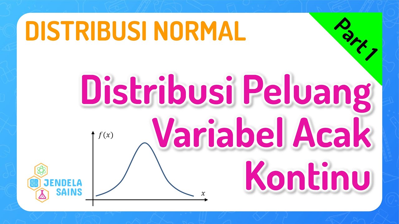
Distribusi Normal • Part 1: Distribusi Peluang Variabel Acak Kontinu

Pertemuan 1 - Distribusi Probabilitas (Part 2)

Random Variables and Probability Mass/Density Functions

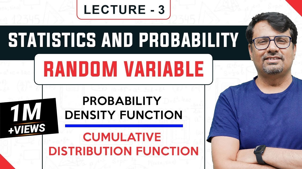
Random Variable, Probability Density Function, Cumulative Distribution Function

Distribusi Binomial • Part 1: Variabel Acak

Discrete random variables | Methods 3 and 4 | MaffsGuru
5.0 / 5 (0 votes)