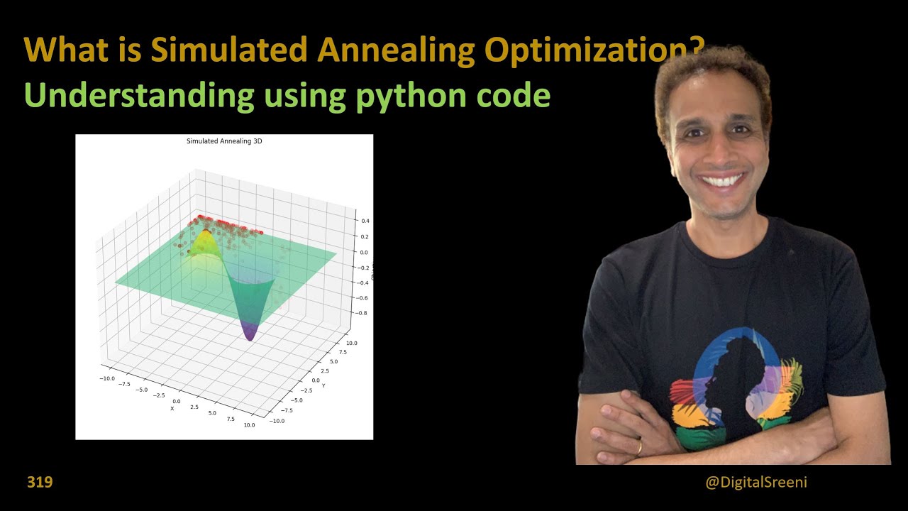
The simulated annealing algorithm explained with an analogy to a toy

Summary

The video explains the simulated annealing algorithm, a method used to solve optimization problems by mimicking the controlled cooling process in metallurgy. It starts with a random configuration and gradually improves it, accepting both good and bad moves depending on a temperature variable that decreases over time. The algorithm is applied to complex problems like the traveling salesman and protein structure design. The video also contrasts simulated annealing with hill climbing and random walk methods, highlighting its balance between exploration and optimization.

Takeaways

• 🔧 The simulated annealing algorithm is inspired by the annealing process in metallurgy, where controlled cooling strengthens metals.
• 🚶 Simulated annealing is widely used in solving optimization problems like the traveling salesman, circuit board design, robot path planning, and bioinformatics.
• 🔄 The algorithm allows for accepting both good and bad moves initially, becoming more selective as it progresses, similar to how we play a water ring game.
• 📊 To apply simulated annealing, we need a way to define the 'energy' or 'fitness' of a solution, which is a measure of how good a configuration is.
• 🎯 The goal is to avoid getting stuck in local minima or maxima and work toward the global optimum solution.
• 💡 The process involves computing the change in energy, represented by delta E, after altering the system's configuration.
• 🌡️ Temperature (T) is a key factor in the algorithm. Initially, the temperature is high, allowing bad moves to be accepted with high probability, and it decreases gradually.
• 📈 As the temperature decreases, the algorithm becomes less likely to accept bad moves, focusing on refining the solution.
• ⚙️ The algorithm repeats this process over several iterations (epochs) with different temperature values, trying to reach the global minimum or maximum.
• 🔍 The parameters like Tmax, Tmin, and number of epochs depend on the specific problem being solved and can be adjusted based on trial and error.

Q & A

What is the origin of the term 'annealing' in the simulated annealing algorithm?

'Annealing' comes from metallurgy, where it refers to a process of slow and controlled cooling to make strong metallic objects. This concept is applied to the simulated annealing algorithm in computer science.

What types of problems can the simulated annealing algorithm be used to solve?

The simulated annealing algorithm is commonly applied to solve problems like the travelling salesman problem, designing printed circuit boards, robot path planning, and in bioinformatics to design 3D protein structures.

How does the water bubble ring toy help explain the simulated annealing algorithm?

The toy illustrates how one might start by pressing buttons vigorously (randomly exploring the solution space), then progressively become more careful and deliberate (moving towards an optimal solution). This mimics the way simulated annealing explores different configurations before narrowing down to a better solution.

How does the simulated annealing algorithm treat bad moves during the optimization process?

In the beginning, the algorithm allows bad moves to explore the solution space, but as it progresses (temperature decreases), the acceptance of bad moves becomes less likely, guiding the algorithm towards better solutions.

What is the role of energy in the simulated annealing algorithm?

Energy (E) measures how good a configuration is in optimization problems. The algorithm computes the energy change (ΔE) between configurations, and this value is used to decide whether to accept a new configuration.

What is a local maximum, and why is it important in the simulated annealing algorithm?

A local maximum is a point in the solution space where the configuration appears optimal but is not the best possible solution (global maximum). The simulated annealing algorithm must avoid getting stuck in local maxima by accepting occasional bad moves early in the process.

How does temperature influence the acceptance of bad moves in the simulated annealing algorithm?

At high temperatures, the probability of accepting bad moves is high, allowing exploration of the solution space. As temperature decreases, this probability lowers, leading the algorithm to focus on good moves and refine the solution.

What happens if the change in energy (ΔE) is very high during the optimization process?

If the change in energy (ΔE) is very high, the probability of accepting the move decreases, indicating a larger difference between the old and new configurations, and the algorithm is less likely to accept the move.

What is the difference between hill climbing and random walk algorithms compared to simulated annealing?

Hill climbing always accepts better moves, making it prone to getting stuck in local maxima. A random walk ignores the quality of moves, leading to endless exploration. Simulated annealing balances exploration and optimization by allowing bad moves initially but becoming selective as the solution progresses.

What are the key parameters in the simulated annealing algorithm, and how are they determined?

The key parameters are maximum temperature (Tmax), minimum temperature (Tmin), and the number of epochs (iterations). Tmax is usually set to a high value (e.g., 3000-5000), Tmin to a low value (e.g., 0-10), and the number of epochs typically ranges from 100 to 200. These parameters are problem-dependent and adjusted based on trial and error.

Outlines

00:00

🔧 Introduction to Simulated Annealing Algorithm

The speaker introduces the concept of simulated annealing, a technique inspired by the annealing process in metallurgy. They explain that annealing involves controlled cooling to create strong metallic objects and how this idea is applied in computer science to solve optimization problems like the traveling salesman, circuit board design, robot path planning, and protein structure modeling.

05:00

🎮 Water Bubble Rings Game as an Analogy

To explain simulated annealing, the speaker uses the water bubble rings game as a metaphor. Initially, players press buttons randomly, but as they get closer to hooking rings, they become more deliberate. This mirrors simulated annealing, where early moves can be random or 'bad,' but later moves become more calculated as the solution improves.

10:01

📊 Configurations and Energy in Optimization

The speaker describes the importance of defining how 'good' a solution is in any problem tackled by simulated annealing. In the water bubble rings game, the fitness of a solution is determined by the number of rings hooked. Similarly, in optimization problems, the system's configuration is measured by its energy level, and changes in this energy (delta E) are used to evaluate moves.

🔄 Local vs Global Maximum and Deadlock

The concept of local maximum is explained through the example of getting stuck with many rings on one hook in the game, leading to a deadlock. This situation represents a local maximum where progress stalls. In optimization, it is crucial to distinguish between local and global maxima and minima to avoid deadlock and move towards the optimal solution.

🔥 Temperature and the Simulated Annealing Process

Simulated annealing involves gradually lowering the temperature, just like in metallurgy, to allow a system to settle into an optimal configuration. At high temperatures, bad moves are accepted more readily to explore solution space, but as the temperature decreases, the algorithm favors only good moves, refining the solution towards the global optimum.

📈 Probability and Accepting Moves

The speaker discusses the probability of accepting moves in simulated annealing. At high temperatures, bad moves are accepted with higher probability, allowing for exploration. As the temperature drops, this probability decreases, limiting the acceptance of bad moves and ensuring the system gradually converges toward the best solution.

🏔️ Hill Climbing vs Random Walk

Two alternative algorithms are discussed: hill climbing, which only accepts good moves and is prone to getting stuck in local minima, and random walk, which explores the solution space indiscriminately and never converges to an optimal solution. Simulated annealing strikes a balance between these extremes by introducing temperature and probability factors.

📉 Configurable Parameters of Simulated Annealing

The speaker emphasizes that key parameters like maximum temperature, minimum temperature, and the number of epochs (iterations) depend on the problem being solved. These parameters need to be adjusted through experimentation to ensure the algorithm avoids local minima and moves toward the global optimum.

🔚 Conclusion

The speaker wraps up by explaining how repeated runs of simulated annealing, adjusting the parameters, help determine whether the solution is heading toward a global minimum or stuck in a local minimum. They conclude by thanking the audience for their attention.

Keywords

💡Simulated Annealing

Simulated annealing is an optimization algorithm inspired by the annealing process in metallurgy. It is used to find approximate solutions to complex problems by gradually reducing randomness (or 'temperature') in exploring possible solutions. In the video, it is described as a method to solve various computational problems, such as the traveling salesman problem, by accepting both good and bad moves initially and becoming more selective as the process progresses.

💡Annealing

Annealing is a process from metallurgy in which materials are heated and then cooled in a controlled manner to improve their properties. The video draws an analogy between this and the simulated annealing algorithm, where the system starts with high randomness (high temperature) and gradually becomes more focused on optimal solutions (cooling) as the temperature decreases.

💡Optimization Problem

An optimization problem is a problem in which the goal is to find the best solution from a set of possible solutions. In the context of the video, problems like designing circuit boards or solving the traveling salesman problem are framed as optimization problems, where simulated annealing helps in finding the 'best' configuration or solution.

💡Energy Landscape

The energy landscape is a metaphor used to describe the set of all possible configurations of a system, with their associated energy levels. Peaks and valleys represent local maxima and minima, which are important in optimization. The goal of simulated annealing, as described in the video, is to find the global minimum (or maximum) without getting trapped in a local minimum.

💡Local Maximum/Minimum

A local maximum (or minimum) is a point in the energy landscape where a solution seems optimal compared to nearby solutions, but it may not be the best overall. In the video, this concept is illustrated by the water bubble game, where focusing too much on one hook can lead to a deadlock, analogous to getting stuck in a local maximum during optimization.

💡Global Maximum/Minimum

The global maximum (or minimum) is the best possible solution in the entire energy landscape. The objective of optimization algorithms like simulated annealing is to find this global solution. In the video, it is mentioned as the desired outcome when maximizing the number of hooked rings in the water bubble game or when solving other optimization problems.

💡Temperature

In simulated annealing, temperature is a controlling parameter that dictates how much randomness or exploration is allowed in the system. High temperatures allow for more exploration, including accepting bad moves, while low temperatures focus on refining the solution. The video uses this concept to explain how the algorithm balances between exploring new solutions and refining existing ones.

💡Energy (E)

Energy (E) represents the 'goodness' or fitness of a solution in an optimization problem. The goal of the simulated annealing algorithm is to minimize or maximize this energy depending on the problem. In the water bubble game example, energy is analogous to the number of rings hooked onto the pegs, with higher energy representing a better configuration.

💡Epoch

An epoch refers to a cycle or iteration in which the simulated annealing algorithm processes solutions at a particular temperature level. The video explains that the algorithm typically runs through hundreds of epochs, gradually reducing the temperature with each one, allowing the system to converge toward a global solution.

💡Hill Climbing

Hill climbing is a simpler optimization algorithm where only moves that improve the solution are accepted, making it prone to getting stuck in local maxima or minima. The video contrasts hill climbing with simulated annealing, highlighting that the latter accepts bad moves early on, reducing the risk of being trapped in suboptimal solutions.

Highlights

Simulated annealing is inspired by the annealing process in metallurgy, which uses slow, controlled cooling to create strong metal objects.

The algorithm is widely applied in problems like the traveling salesman problem, printed circuit board design, robot path planning, and protein molecule structure design in bioinformatics.

The game analogy helps explain the concept of simulated annealing: at first, you play randomly and accept bad moves, but as you get closer to the solution, you become more deliberate and careful.

At the beginning of the algorithm, bad configurations are accepted, but as the solution progresses, only good moves are selected to reach the final goal.

To apply simulated annealing, you need a way to measure how good a configuration is. This is often described as the 'energy' or 'fitness' of the system.

Energy (E) of the system is computed for each configuration, and the change in energy (ΔE) is calculated when a new configuration is introduced.

In optimization problems, local maxima or local minima can occur, where a solution seems optimal but is not the global best.

Global maxima or minima represent the true optimal solution, while local optima can trap the system in suboptimal configurations.

The algorithm starts with a high temperature (Tmax) and gradually cools down to a low temperature (Tmin), simulating the annealing process in metallurgy.

At high temperatures, the probability of accepting bad moves is high, allowing exploration of the solution space. As the temperature lowers, the probability decreases, leading to more selective moves.

If a new configuration improves the system's energy (ΔE is positive), it is accepted. If it worsens the energy (ΔE is negative), it may still be accepted with a certain probability, depending on temperature.

The number of iterations (epochs) and temperature values (Tmax and Tmin) are parameters that need to be set based on the problem being solved.

Simulated annealing strikes a balance between two extremes: hill climbing, which only accepts better moves and is prone to getting stuck in local optima, and random walk, which explores without considering solution quality.

Hill climbing is a greedy algorithm that always goes toward better solutions but risks getting stuck in local minima.

Random walk, by contrast, explores the space without caring about the quality of moves, but it never converges to the best solution.

Transcripts

Today I will explain the simulated

annealing algorithm. The word annealing

comes from metallurgy. In metallurgy, to make

really strong metallic objects, people

follow a slow and controlled cooling

procedure known as annealing. The same can

be applied to computer science algorithms

The simulated annealing algorithm is widely

applied to solve problems like

travelling salesman problem, designing

printed circuit boards, for planning of a

path for a robot, and in bioinformatics

to design three-dimensional structures

of protein molecules. To better explain

algorithm I have here with me

our toy game known as water bubble rings.

So this is a small water container that

has these plastic rings inside and has

some hooks as well.

It also comes with these two buttons

which can be pressed, so when we press

the buttons, the rings move inside the water.

Obviously the objective in this game is

to get as many rings hooked as we can.

So, how does someone play this game?

If we were to play it how would we play it?

Intuitively, we would first start by pressing the

buttons vigorously and by checking to

see if we can get all rings hooked or

checking to see as many see if we can

get as many rings hooked as we can

without worrying about the solution so

that's how we would start and once we

have some rings hooked in the hooks, we will

be more careful after that, we will be more

deliberate and we'll play it more

seriously, as we get closer to the final

solution, we will be very careful very deliberate

and out final moves will be extremely carefully planed

so that's the intuition behind the simulated annealing algorithm

At the beginning you don't care

if you are

actually moving towards the good solution and you

accept bad moves as well, you accept

bad configurations as well but as you

progress towards the solution we become

more careful and we try to get closer to

the solution and by selecting only the good

moves. So to formulate any problem in order

to apply algorithms like simulated

annealing every problem needs to have a

way to define how good a given

configuration is. So, for this particular

game, for this particular toy, given a

configuration of this toy, we can tell how

good the solution is by checking the

number of rings that are hooked, right?

So every system or every problems that

you're solving needs to have a way to

describe the goodness or the fitness of

the solution for the problem. In other

words we need to, in optimization problems,

also known as energy of the solution, in

other words we need to have a mechanism

to define the energy of the system. So if

E is the energy of the system we represent

the energy using E, and once we have

a mechanism to compute E, you can also compute

delta E or change in energy. So every time

the system goes through a change of

configuration, we can compute the

change in energy.

Now, talking about this game, when

somebody's playing this game one

can play it in a specific way

so someone can focus in just one of the

hooks and continue to play the game so

that he or she can get as many rings as

possible in one of the holes, forgetting

about the remaining hooks. Now if we play

like that, after a certain time, we will end

up in a deadlock where we have a lot of

rings hooked in one of the hooks but

the other hooks are empty. At that point if you

play vigorously you will you will

remove lot of the rings which are already solved

and you play it very slow it will take a

really long time to get to the final solution. So,

situations like that in optimization

problems are known as a local maximum or

local minimum, so you were to plot

all possible configurations of a given

system in X axis and in Y axis we were to compute

the corresponding energy of all the

configurations than energy landscape

usually looks something like this so

high values correspond to maximum energy in our

case since we want maximum number of

rings to be hooked

it's a maximization problem and we want

the maximum value of energy for our

problem and places like these in the

energy landscape which look like we have

to look like

hi value in energy but which actually

take us to the deadlock are known as a

local maximum or if you are trying to

minimize the energy that these are also

known as local minimum. And the actual energy

that we want or the configuration that we want

and the maximum energy is known as a

global maximum, if we're trying to

find the maximum. So this is something that we

need to become vigilant about when applying

algorithms like these to solve the problem is a

to be careful and to check if we are

actually being stuck in a local minima

but we're actually getting closer to the

the global maxima or global minimum. Now, once we have

a way to define energy once and once we

know about global minima an global maxima, we

also need a way in which we can change

the configuration of the system every

time so in the water bubble rings game

in this toy, we can change the

configuration by placing the

button, so it randomly alters the

configuration of the system so that we

get a new configuration. So every problem

that we apply algorithm like this

needs to have a mechanism to alter

the configuration and so you see the

current configuration, we need to have a

mechanic to alter the current configuration

to the next configures and and usually

this is this is also known as making a move

in the water bubble rings we

make it just by pressing the button

So, once we have the these definitions laid out

now I would like to explain the

simulated annealing algorithm

So the idea is to start with the initial configuration

or given random configuration

Then, we use introduce a variable

known as temperature. Just the way in

case of annealing we start with initial

high temperature and we slowly

controlled cool the material, for the algorithm

we start with a maximum temperature

Tmax, and this is a monotonic

decreasing function that slowly

decreases to Tmin, or minimum temperature

so whatever value of temperature we

first compute the current energy of the

system, for the current configuration C

using E(C), then we change the

configuration or alter the configuration

a little bit using the technique for

altering the configuration and then we

get the new configuration and we compute

the energy for this new configuration

Once we have EC and EN, we can compute

Delta E or change in energy and so

now we have old configuration C or the

current configuration C and see the new

configuration N and we know that

change in energy. Since we are working on

a maximization problem if delta E is

positive or the change in energy is a

good one, or if it's a good move

we accept the move. In other words we set

the next configuration to the current

configuration and we accept the move, and we

repeat the process so so that we are

getting closer to the we're getting a

better solution, and move close to the

final solution. At every step,

if we see that change in energy is

negative or in other words, if we are

making a bad move then what do we do?

In cases like these, we compute this

probability, I will give the details of this,

but we compute the probability of

this and then if we see that the

probability is very high then we accept

the move even if it is a bad more and if

the probability is low, then we have low

probability to accept the bad move. So this

probability depends on these two variables

change energy delta E and the

temperature factor T. When

temperature is very high then the

probability for accepting the bad move

becomes very high, in other words, at high

temperatures we are exploring the solution

space or we are exploiting the

configurations and we're accepting

bad moves as well, and when the temperature

is low this probability becomes very

low and we have very low probability to

accept bad moves. Say, for instance when

temperature is very high, say 10,000 and

change in energy is not very high, say 100 or 10

then this whole thing computes to a

a small negative number

e to the power small negative number gives you

something very close to one and a number

that is close to one has a very high (correction)

probability to become greater than a

random number between 0 and 1, which means we get

a very high probability, so when temperature

is very high

we have high probability to accept bad

moves as well. Now, we also see that the change

in energy, delta E also influences it, so if

that change in energy is really high

we are again have a low probability to

accept the move and when the change in energy is

small we have a high probability to accept the move.

So this is how the whole algorithm works

So, we repeat the process

for certain number of times

usually known as the number of epochs, usually 100 to 200 times

and for every value of temperature

we repeat the process and finally expecting

the solution to converge towards the

global minimum. So that's the idea behind

the algorithm. Now on either extremes are 2 other algorithms

known as hill climbing and

random walk. So if we remove the

probability factor or the temperature

factor and always accept the good moves only

then that's hill climbing

or it's like a greedy algorithm which always go

towards a better solution. Such, algorithms are

prone to easily be stuck in local minima.

On the other end is a random walk which

means, we don't care about

how good a move we are making every time but we

just explore, continue to explore, the space

Such algorithms never converge and

will probably never give you the best

optimal solution. Now the parameters Tmax

Tmin, and number of epoch are dependent on

the problem that we are solving, usually

we start with high temperatures like a

few thousands, let's say 3000 or 5000 and then

the minimum temperature is set to a small value like 0 or 10

or something like that. Number of epoch is usually

a hundred, or 200 depending on the problem

so these are the parameters that you can

explore by applying the algorithm to

problem that we have, and if you run it

multiple times you will have an idea of whether

you're being stuck in the local minima or

you're heading towards the global minimum

thank you