The Empirical Rule
Summary
TLDRThe video script explains the Empirical Rule, which is used for visualizing data with a bell-shaped distribution. It highlights that approximately 68% of data falls within one standard deviation, 95% within two, and 99.7% within three standard deviations from the mean. The rule is significant as it allows for the estimation of the bell curve's shape using just the mean and standard deviation. The script also demonstrates how to apply the Empirical Rule to a dataset with a mean of 50 and a standard deviation of 10, showing that the rule can accurately predict data distribution, provided the data is normally distributed.
Takeaways
- 📊 The Empirical Rule is a method to visualize data distribution when it is assumed to be bell-shaped or normally distributed.
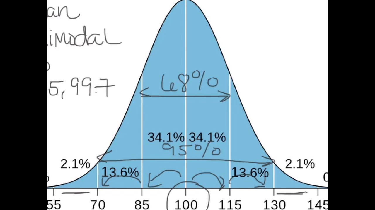
- 🔢 According to the Empirical Rule, 68% of data points fall within one standard deviation of the mean.
- 📉 About 95% of data points are within two standard deviations of the mean in a normal distribution.
- 📈 Almost all (99.7%) data points (with a few exceptions) are within three standard deviations of the mean.
- 📋 For a dataset with a mean of 50 and a standard deviation of 10, 68% of observations would be between 40 and 60.
- 📐 The Empirical Rule helps to estimate the shape of the bell curve using only the mean and standard deviation.
- 📈 When drawing the bell curve, the tails are drawn with different slopes to represent the data distribution outside of one, two, and three standard deviations.
- 📊 The distribution under the curve is such that 34% of data is within one standard deviation on each side of the mean, 13.5% between one and two standard deviations, and 2.5% in the outermost tails.
- 👤 The Empirical Rule can be applied to any dataset where the mean (μ) and standard deviation (σ) are known, and the distribution is assumed to be normal.
- 🗂️ The Empirical Rule is particularly useful for creating a rough sketch of the histogram based on just two numerical values, enhancing our understanding of data distribution.
Q & A
What is the Empirical Rule?
-The Empirical Rule is a guideline used to visualize the distribution of data when it is assumed to be bell-shaped or normally distributed. It states that approximately 68% of the data falls within one standard deviation of the mean, 95% within two standard deviations, and 99.7% within three standard deviations.
How does the Empirical Rule improve upon Chebyshev's Rule for normal distributions?
-Chebyshev's Rule provides a rough estimate of data distribution for any dataset, but for normal distributions, it can be too broad. The Empirical Rule offers a more precise visualization of the distribution by using the specific properties of bell-shaped distributions, allowing for a more accurate representation based on the mean and standard deviation.
What percentage of data is expected to fall within one standard deviation of the mean in a normal distribution?
-According to the Empirical Rule, approximately 68% of the data is expected to fall within one standard deviation of the mean in a normal distribution.
What does it mean for a distribution to be bell-shaped?
-A bell-shaped distribution, also known as a normal distribution, is symmetrical and centered around the mean, with the data points decreasing in frequency as they move away from the mean, resembling the shape of a bell.
How can you determine the shape of the bell curve using the Empirical Rule?
-By knowing the mean and standard deviation, you can determine the shape of the bell curve using the Empirical Rule. You plot the values at one, two, and three standard deviations from the mean and draw the curve with the appropriate slopes and widths to reflect the percentages of data within those ranges.
What percentage of the data is outside of three standard deviations in a normal distribution?
-In a normal distribution, only about 0.3% of the data falls outside of three standard deviations from the mean.
How does the Empirical Rule help in visualizing the tails of a normal distribution?
-The Empirical Rule helps visualize the tails of a normal distribution by indicating that 5% of the data is outside of two standard deviations and 32% is outside of one standard deviation. This information allows for the correct drawing of the tails with increasing slopes towards the center.
What is the significance of the percentages 34%, 13.5%, and 2.5% in the context of the Empirical Rule?
-These percentages represent the distribution of data under the bell curve: 34% of the data is within one standard deviation on either side of the mean, 13.5% is between one and two standard deviations on either side, and 2.5% is outside of two standard deviations but within three standard deviations on either side.
Can the Empirical Rule be applied to any type of data distribution?
-No, the Empirical Rule can only be applied to data distributions that can be assumed to be normal or bell-shaped. It does not apply to skewed or other non-normal distributions.
How can the Empirical Rule be validated using a real dataset?
-The Empirical Rule can be validated by applying it to a dataset with a known mean and standard deviation and then comparing the predicted percentages within one, two, and three standard deviations to the actual data distribution, such as through a histogram.
What is the importance of knowing the mean and standard deviation in the context of the Empirical Rule?
-Knowing the mean and standard deviation is crucial for the Empirical Rule because these two numbers alone enable the accurate visualization of the data's distribution shape, providing a clear understanding of how the data is spread around the mean.
Outlines

This section is available to paid users only. Please upgrade to access this part.
Upgrade NowMindmap

This section is available to paid users only. Please upgrade to access this part.
Upgrade NowKeywords

This section is available to paid users only. Please upgrade to access this part.
Upgrade NowHighlights

This section is available to paid users only. Please upgrade to access this part.
Upgrade NowTranscripts

This section is available to paid users only. Please upgrade to access this part.
Upgrade NowBrowse More Related Video

Normal Distributions Explained – With Real-World Examples
What is a Bell Curve or Normal Curve Explained?
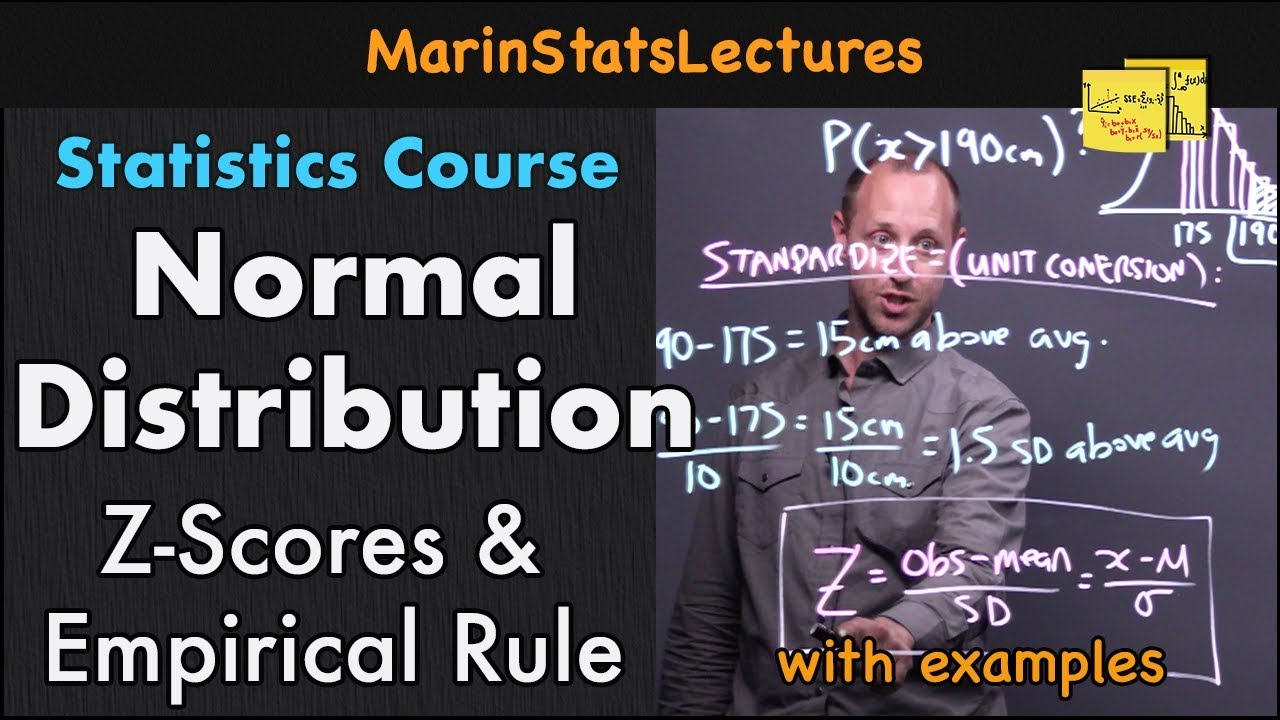
Normal Distribution, Z-Scores & Empirical Rule | Statistics Tutorial #3 | MarinStatsLectures
Peluang Distribusi NORMAL beserta Contoh Soal Pembahasan

Normal Distribution and Empirical Rule
Statistics for Psychology
5.0 / 5 (0 votes)