Deriving Kinematic Equations - Kinematics - Physics
Summary
TLDRIn this video, you will learn how to derive the four key kinematic equations using a velocity versus time graph. The instructor guides you through the derivation process step-by-step, starting with the relationship between slope and acceleration, then progressing through calculating displacement by analyzing the area under the graph, and finally deriving the equations for velocity and displacement under constant acceleration. The video concludes with a recap of all four equations and a preview of the next lesson, which will cover a useful chart for applying these equations to solve problems.
Takeaways
- 📈 The script explains the derivation of the four kinematic equations using a velocity versus time graph.
- 🔍 The slope of the line on the velocity-time graph represents acceleration, calculated as the change in velocity over time.
- ✏️ The first kinematic equation is derived as \( v_f = v_i + a \cdot t \), where \( v_f \) is the final velocity, \( v_i \) is the initial velocity, and \( a \) is the acceleration.
- 📏 The second equation is derived from the area under the velocity-time graph, representing displacement, and is given by \( \Delta x = v_i \cdot t + \frac{1}{2} a \cdot t^2 \).
- 🔢 The third kinematic equation relates average velocity to displacement and time, and is expressed as \( \Delta x = \frac{v_f + v_i}{2} \cdot t \).
- 🔄 The fourth equation is derived by manipulating the third equation and is written as \( v_f^2 = v_i^2 + 2a \cdot \Delta x \).
- 🔄 The script emphasizes that these equations are applicable for scenarios with constant acceleration.
- 📚 The script mentions that the next video will provide a kinematics chart to help decide which equation to use for different problems.
- 📉 The area under the curve in the velocity-time graph is broken down into a rectangle and a triangle to derive the second kinematic equation.
- 📐 The script uses algebraic manipulation to derive the third and fourth kinematic equations from the first and second equations.
Q & A
What is the first kinematic equation derived from the video?
-The first kinematic equation is \( v_f = v_i + a \cdot t \), where \( v_f \) is the final velocity, \( v_i \) is the initial velocity, \( a \) is the acceleration, and \( t \) is the time.
How is acceleration represented on a velocity versus time graph?
-Acceleration is represented as the slope of the line on a velocity versus time graph, calculated as the change in velocity divided by the change in time.
What does the area under the velocity versus time graph represent?
-The area under the velocity versus time graph represents the displacement of an object.
What is the second kinematic equation?
-The second kinematic equation is \( \Delta x = v_i \cdot t + \frac{1}{2} a \cdot t^2 \), which combines the area of a rectangle and a triangle under the velocity-time graph.
How is the average velocity calculated in the context of the third kinematic equation?
-The average velocity is calculated as the displacement divided by the change in time, or equivalently, as the average of the initial and final velocities when acceleration is constant.
What is the third kinematic equation?
-The third kinematic equation is \( \Delta x = \frac{v_f + v_i}{2} \cdot t \), which relates displacement to the average velocity, initial velocity, final velocity, and time.
How is the fourth kinematic equation derived?
-The fourth kinematic equation is derived by manipulating the third equation to solve for \( v_f^2 \), resulting in \( v_f^2 = v_i^2 + 2a \cdot \Delta x \).
What is the significance of the equation \( v_f^2 = v_i^2 + 2a \cdot \Delta x \)?
-This equation is significant as it relates the final velocity squared to the initial velocity squared, acceleration, and displacement, which is useful for problems involving constant acceleration.
Why is it important to consider constant acceleration when using the kinematic equations?
-The kinematic equations are derived under the assumption of constant acceleration. If acceleration is not constant, these equations may not accurately describe the motion.
What is the purpose of a kinematics chart mentioned in the video?
-A kinematics chart helps to decide which kinematic equation to use for a particular problem by providing a visual guide based on the given information in the problem.
What common issue do students face with the kinematic equations, as mentioned in the video?
-Students often struggle to determine which kinematic equation to use for a given problem, which is why a kinematics chart is recommended for assistance.
Outlines

This section is available to paid users only. Please upgrade to access this part.
Upgrade NowMindmap

This section is available to paid users only. Please upgrade to access this part.
Upgrade NowKeywords

This section is available to paid users only. Please upgrade to access this part.
Upgrade NowHighlights

This section is available to paid users only. Please upgrade to access this part.
Upgrade NowTranscripts

This section is available to paid users only. Please upgrade to access this part.
Upgrade NowBrowse More Related Video
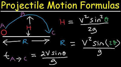
Introduction to Projectile Motion - Formulas and Equations

Kinematic Equations for Linear Motion (Clip) | Physics - Kinematics
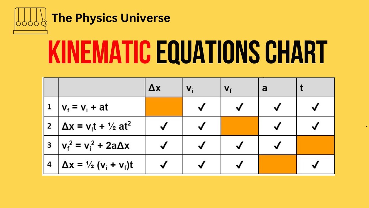
Creating And Using Kinematic Equations Chart - Kinematics - Physics
Acceleration and Kinematic Equations | Physics in Motion
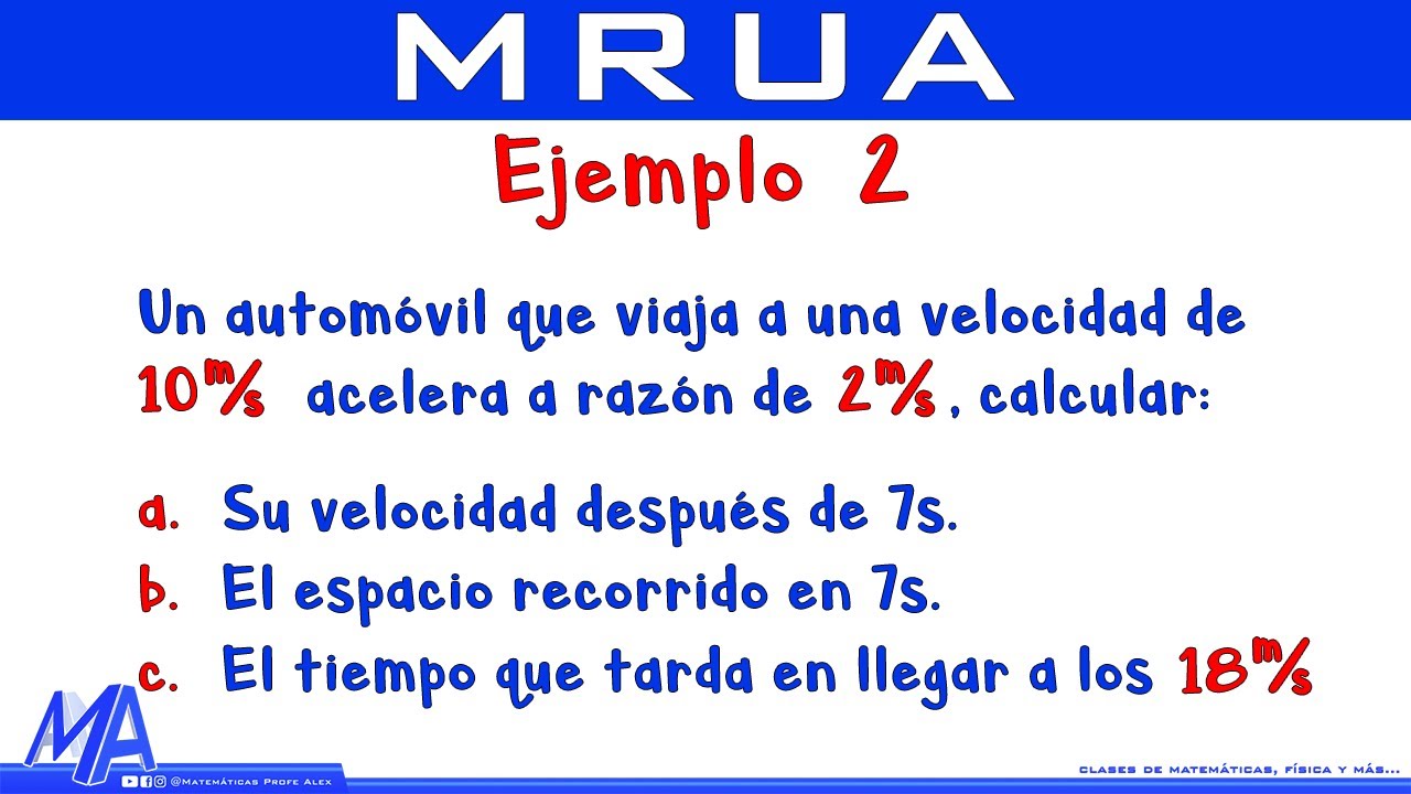
Movimiento Rectilíneo Uniformemente Acelerado o Variado MRUA MRUV | Ejemplo 2

Kinematic Equations in One Dimension | Physics with Professor Matt Anderson | M2-04
5.0 / 5 (0 votes)