Calculus - Approximating the instantaneous Rate of Change of a Function
Summary
TLDRThe video script delves into the concept of instantaneous change in a function, contrasting it with average change by focusing on a single point rather than between two. It illustrates the process of approximating this change by moving a second point closer to the point of interest, observing how the average rate of change converges to a limiting value. This method provides a practical way to estimate the instantaneous rate of change, such as the speed of a rocket or population growth rate, despite its approximation nature. The script teases the introduction of calculus' limits as a more precise tool for future lectures, encouraging viewers to explore further.
Takeaways
- 📈 The concept of instantaneous change in a function is introduced as a way to describe how a function changes at a single point, rather than over an interval.
- 🔍 The distinction between instantaneous and average change is highlighted, with the former focusing on a specific point and the latter considering a range.
- 🚀 Instantaneous change can be applied to real-world situations like the speed of a rocket immediately after launch or the rate of population growth.
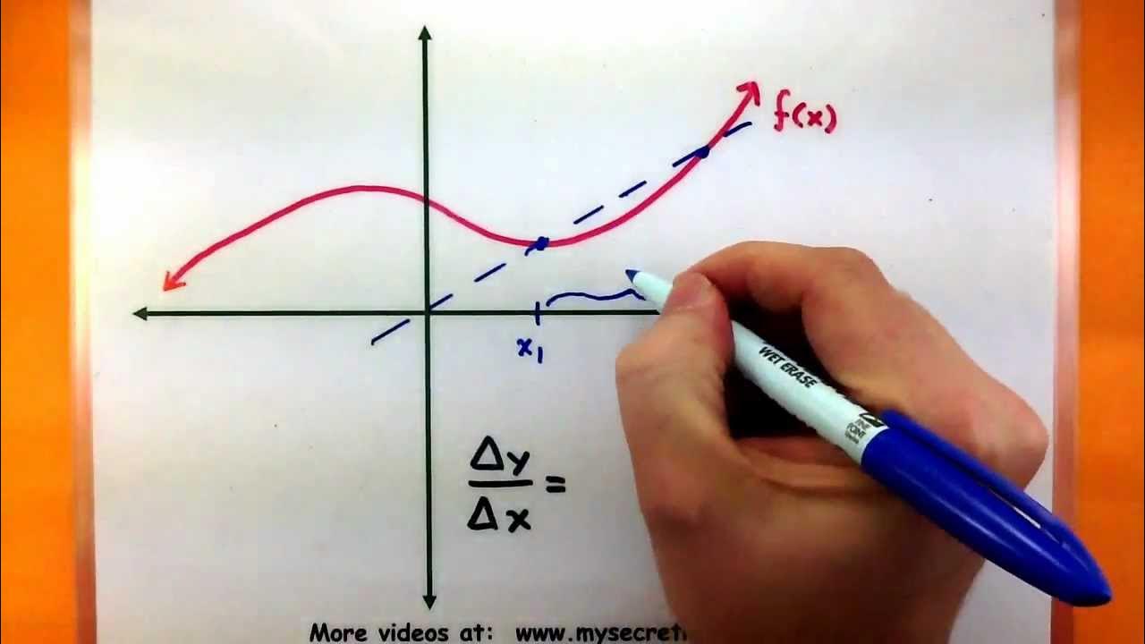
- ❌ The traditional method of finding change using two points results in a 0/0 indeterminate form when trying to apply it to a single point.
- 🔑 The secret to finding change at a single point is to cleverly use the average rate of change and then take a limit as the points converge.
- 📐 The process involves choosing two points, calculating the average rate of change, and then moving the second point closer to the first to observe changes in the rate.
- 📉 As the second point approaches the first, the average rate values converge towards a limiting value, which is an approximation of the instantaneous rate of change.
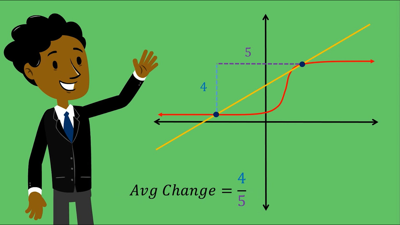
- 📊 The example provided demonstrates the process of moving a point closer and observing the average rate of change values approach a specific number, indicating a limiting value.
- 🤔 While the limiting value provides a good approximation, it is not exact, and there is a need for a method to determine the exact value the rate is approaching.
- 🧠 Calculus introduces the concept of a limit, which is a tool designed to find the exact value a function approaches, providing a solution to the problem of approximation.
- 📚 The script encourages viewers to look forward to the next lecture on limits and to explore more examples of approximating instantaneous rates of change on the provided website.
Q & A
What is the main concept discussed in the script?
-The main concept discussed in the script is the idea of instantaneous change of a function, which is the rate of change at a single point rather than between two points.
Why is it difficult to describe the change of a function at a single point using the usual method?
-It is difficult because the usual method requires two points to calculate the change in both the y and x directions. At a single point, it appears there is no change in either direction, leading to a 0/0 indeterminate form when attempting to use the change formula.
What is the alternative method to describe the change at a single point?
-The alternative method is to use the average rate of change between two points and then move the second point closer and closer to the first point, observing how the average rate of change approaches a limiting value.
What is the term used to describe the value that the average rate of change approaches as the second point gets closer to the first point?
-The term used is 'limiting value,' which serves as an approximation to the instantaneous change of a function.
Can the limiting value be considered an exact measure of the instantaneous rate of change?
-No, the limiting value is an approximation because there is no precise way to determine how close to the limiting value the average rate of change is getting.
What does the script suggest as a more exact method for finding the limiting value?
-The script suggests that the concept of 'limit' in Calculus provides a more exact method for finding the limiting value that a function approaches.
What is an example of a real-world application of finding the instantaneous rate of change?
-An example given in the script is finding the instantaneous speed of a rocket a few minutes after launch or the instantaneous rate of change of a population.
What is the process of finding the limiting value in the context of the script?
-The process involves selecting a point on the function and another point, calculating the average rate of change between them, and then repeatedly moving the second point closer to the first point while recording the new average rate of change until a consistent limiting value is approached.
What is the significance of the number 2 in the example provided in the script?
-The number 2 is the limiting value that the average rate of change seems to be approaching as the second point gets closer to the first point, indicating the instantaneous rate of change at that specific point on the function.
How does the script suggest we can improve our understanding of the instantaneous rate of change?
-The script suggests that by moving the points closer together and observing the changes in the average rate of change, we can gather more evidence and improve our understanding of the instantaneous rate of change, even without the exact mathematical concept of a limit.
Outlines
🚀 Understanding Instantaneous Change
This paragraph introduces the concept of instantaneous change in a function, contrasting it with average change by emphasizing the need to describe the change at a single point rather than between two points. It discusses the limitations of using the change formula for a single point, which results in an indeterminate form of 0/0. The solution to this problem is hinted at by using the average rate of change in a clever way, setting the stage for the concept of limits in calculus.
📏 Approximating Instantaneous Change with Average Rate
The paragraph explains the process of approximating the instantaneous rate of change by starting with two points and calculating the average rate of change between them. As the second point is moved closer to the first, the average rate values are recorded and are expected to converge to a limiting value. This limiting value serves as an approximation for the instantaneous change of the function at a specific point. An example is provided to illustrate this process, showing how the average rate values approach a limiting value as the points are brought closer together.
🔍 The Limiting Value and Its Significance
This section delves deeper into the concept of the limiting value, which is the value that the average rate of change approaches as the points converge. It discusses the idea that while the limiting value can be used as an approximation for the instantaneous rate of change, it is not exact due to the inability to determine how close the values are to the true limit. The paragraph also introduces the notion that calculus provides a tool, the limit, to find this exact value, which will be discussed in future lectures.
🔧 The Practicality of Average Rate of Change
The paragraph highlights the practical use of the average rate of change to understand the function's behavior at a single point, even without the formal concept of limits. It emphasizes that by moving the points closer and closer, one can get a good approximation of the instantaneous rate of change. Additionally, it encourages viewers to explore more about this topic through examples and future lectures on limits.
📚 Engaging with the Content and Further Resources
The final paragraph serves as a call to action for viewers to engage with the content by liking and subscribing to the channel. It also invites viewers to explore more about the topic through additional examples and the next lecture on limits. The paragraph provides a resource for further learning by directing viewers to the creator's website, MySecretMathTutor.com, and concludes with a thank you note for watching.
Mindmap
Keywords
💡Instantaneous Change
💡Average Change
💡Single Point
💡0 Divided by 0
💡Average Rate of Change
💡Limiting Value
💡Instantaneous Rate of Change
💡Approximation
💡Limit (in Calculus)
💡MySecretMathTutor.com
Highlights
The concept of instantaneous change in a function is introduced, emphasizing the need for a single point analysis rather than between two points.
Instantaneous change can be applied to scenarios such as the speed of a rocket post-launch or the rate of population change.
The traditional method of describing function change requires two points, which is not applicable for instantaneous change.
Attempting to use the change formula for a single point results in an indeterminate form of 0/0.
A clever method is introduced to approximate change at a single point using the average rate of change between two points.
The process involves moving the second point closer to the first, recording the average rate of change as it converges to a limiting value.
An example demonstrates the process of finding the instantaneous rate of change by moving the second point closer to the first.
The average rate of change is measured between two points, initially yielding a value of 1.
As the second point is moved closer, the average rate increases, suggesting a trend towards a specific limiting value.
The values of the average rate of change approach a limiting value of 2, indicating the instantaneous rate of change.
The approximation of the instantaneous rate of change is limited by the inability to determine how close to the limiting value we are.
Calculus provides a tool called 'limit' to find the exact value a function approaches, which is introduced as a solution to the approximation issue.
The limit is presented as a fundamental tool in Calculus for future problems, to be discussed in the next lecture.
Even without the limit, the average rate of change can be used to approximate the instantaneous change at a single point.
The importance of moving points closer together to find the limiting value for a more accurate approximation is emphasized.
The video concludes with an invitation to like and subscribe for more content on approximating instantaneous rates of change.
The presenter also promotes their website, MySecretMathTutor.com, for additional resources and information.
Transcripts
When it comes to the instantaneous change of a function, our goal is to describe how
a function is changing. The difference between instantaneous change
and average change is that we want to describe the change using only a single point, rather
than between two points. This can be used for things like the instantaneous
speed of a rocket a few minutes after launch, or possibly the instantaneous rate of change
of a population.
One problem we run into is that when we normally describe something like the change of a function
we usually need two points to do it. This is so we can record both the change in
the y-direction and x-direction.
If we are at a single point, then it doesn't seem like we are changing in either direction.
To see this you might attempt to use our change formula for a single point.
This unfortunately would give you 0 divided by 0, which isn't really useful for describing change.
Fortunately there is a way we can find the change at a single point, and the secret
is in using the average rate but in a very clever way!
Let's see how this is done. To approximate the change at a single point
we begin by chosing a point, along with one other point.
This gives us two points. Using these two points we find the value of the
average rate of change between them.
Now rather than stopping there, we instead start moving the second point closer
and closer. Each time we do this we can record the new
value for the average rate between them. Our hope is that as we find these new values,
they will begin to get closer and possibly settle on some specific value.
This is what we will call our limiting value, and it works great as an approximation to
the instantaneous change of a function.
Let's take a look at a simple example to see this process in action.
Here we have a function, and I want to know the instantaneous rate
of change at this point here. I'll choose it, along with one other point.
Now I can measure the average rate of change between these two points, using my average
rate formula. And when I do I get a value of 1.
Now let's move that second point a bit closer. If I measure the average rate now, I get a
value of 1.5 Let's move it closer again. This time the
value is 1.8
As we continue to move this second point, we are getting different values for the rate
of change. Even though they are changing, they seem to
be getting close to a limiting value. In fact it appears they are getting close
to the number 2
Let's move them closer still to see if this is the case!
After moving them really close together, our value for the average rate is now 1.99, and
that's really close to 2, and even more evidence that our limiting value is indeed 2.
Since we are looking at the average rate, and moving the point closer,
2 can be considered an approximation for the instantaneous rate of change of our function.
It otherwords, it gives us a great way to describe how the function is changing at a
single point, which is exactly what we want!
Unfortunately, we can only call it an approximation. This is because we don't have any way of precisely
saying how close to the value of 2 we are getting.
Maybe the true value its approaching is 2.015, or it might even be approaching 1.993.
We can move these points closer together to gather more evidence,
but it would be much better if we had an an exact way of knowing what value this rate
was approaching, a method for finding the limiting value, exactly.
Fortunately Calculus has an answer for this issue, and its one of the first major tools
we'll need for many future problems. This tool is known as the limit, and it's
job is to help us describe what value a function is approaching, exactly.
We'll save this for the next lecture. For now its good to recognize that even without
the limit, we can still get a very good idea of how the
function is changing at a single point, we simply use our average rate of change and
then move our points closer and closer together so we can find that limiting value.
Thanks for watching.
Hey, did you enjoy this video? Don't forget to like it, and then subscribe to my channel!
If you want to know more about approximating the instantaneious rate of change, you can
watch a few of my examples. You can also move onto my next lecture where
I talk about one of the most powerful tools of Calucus, the limit!
For some of my other videos, don't forget to visit my web site: MySecretMathTutor.com
Thanks again for watching!
Посмотреть больше похожих видео
5.0 / 5 (0 votes)