SOAL & PEMBAHASAN MS.EXCEL || FUNGSI STATISTIKA

Summary

This tutorial demonstrates how to use various Excel functions to analyze and manipulate student grade data. The video guides viewers on how to compute totals, averages, highest, and lowest scores for both IPA and Informatika subjects. Specific formulas like SUM, AVERAGE, MAX, MIN, and COUNT are explained for each cell in the table, with special attention given to calculating the statistics for an individual student, Cahaya Pratiwi. Additionally, the video showcases how to quickly use the AutoFill feature to apply these formulas across multiple rows, enhancing efficiency in data analysis.

Takeaways

• 😀 The script provides instructions on using Excel functions to calculate various statistics (e.g., total, average, highest, lowest) for student scores in different subjects.
• 😀 Excel columns are labeled with letters (A, B, C...) and rows with numbers (1, 2, 3...), and it is essential to identify them when working with formulas.
• 😀 The `SUM` function is used to calculate the total value in a range of cells, such as the total IPA (science) or Informatics scores of all students.
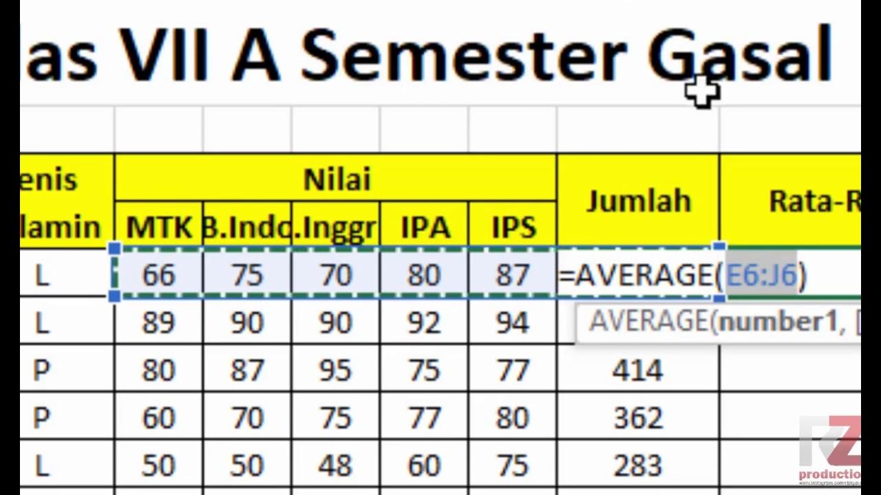
• 😀 The `AVERAGE` function helps to calculate the average score for a specific subject (IPA or Informatics) across all students.
• 😀 The `MAX` function is used to find the highest score in a given range, such as the highest IPA or Informatics score among students.
• 😀 The `MIN` function is used to determine the lowest score in a given range, such as the lowest IPA or Informatics score among students.
• 😀 The `COUNT` function is used to count the number of data entries, which helps in finding the number of students or data points for a specific subject.
• 😀 For individual student data, the formulas focus on specific cells (e.g., D6 for IPA and E6 for Informatics) for calculating sums, averages, highest, and lowest values.
• 😀 The AutoFill feature in Excel allows you to quickly copy formulas down a column, making it easier to apply the same calculation to multiple rows (e.g., calculating the highest score for students 2-5).
• 😀 To calculate the highest score for a specific range (e.g., from H7 to H10), you can first calculate the highest score for one student and use AutoFill to apply the same formula to other students' rows.

Q & A

What is the first step in answering the Excel-related questions in the script?

The first step is to identify the columns and rows involved in the table. For this specific case, the columns range from B to J, and the rows range from 5 to 14.

How do you calculate the total IPA scores for all students?

To calculate the total IPA scores, you use the formula `=SUM(D6:D10)` where D6 to D10 contains the IPA scores of all the students.

What is the formula used to calculate the total Informatics scores?

The formula used to calculate the total Informatics scores is `=SUM(E6:E10)` where E6 to E10 contains the Informatics scores of all the students.

How do you calculate the average IPA score?

The average IPA score is calculated using the formula `=AVERAGE(D6:D10)`, which averages the values in the range D6 to D10.

What is the formula for calculating the maximum IPA score?

To calculate the maximum IPA score, the formula `=MAX(D6:D10)` is used, which finds the highest value in the range D6 to D10.

How do you calculate the minimum Informatics score?

To calculate the minimum Informatics score, the formula `=MIN(E6:E10)` is used, which finds the lowest value in the range E6 to E10.

What should be the formula to calculate Cahaya Pratiwi's total grades in both subjects?

To calculate Cahaya Pratiwi's total grades, use the formula `=SUM(D6:E6)`, which sums the values of her IPA (D6) and Informatics (E6) scores.

How do you calculate Cahaya Pratiwi's average score?

Cahaya Pratiwi's average score is calculated using the formula `=AVERAGE(D6:E6)`, which averages her IPA and Informatics scores.

What is the procedure to find the highest value for students from H7 to H10 using Autofill?

First, calculate the highest value for the first student using `=MAX(D6:E6)`. Then, use the Autofill feature by clicking on the cell containing the formula (e.g., H6) and dragging it down to H10 to quickly fill the remaining cells with the highest values for other students.

How do you calculate the total number of data points for Cahaya Pratiwi?

To calculate the total number of data points for Cahaya Pratiwi, use the formula `=COUNT(D6:E6)` which counts the number of cells containing data in the range D6 to E6.