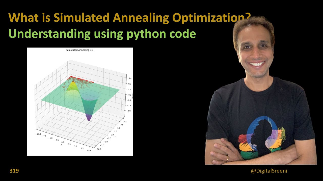
Simulated Annealing

Summary

This video explores the limitations of hill climbing in optimization and introduces simulated annealing as a solution. The speaker explains how hill climbing struggles with local maxima and how simulated annealing overcomes this by sometimes allowing worse moves, mimicking the metallurgic process of heating and cooling metals. By controlling the randomness of these decisions, simulated annealing helps find better solutions over time, eventually narrowing down to the optimal one. The video delves into the math behind this method and demonstrates how it works with temperature decline and probability.

Takeaways

• 🤔 Hill climbing struggles with local maxima, where it won't accept worse moves, potentially trapping it.
• 🎲 Introducing controlled randomness allows for sometimes making worse moves to escape local maxima.
• 🌱 Metaheuristics are inspired by natural processes and provide solutions beyond simple optimization algorithms.
• 🔥 Simulated annealing is inspired by metallurgical processes, where heated metal gradually cools to a stable structure.
• 🌡️ Simulated annealing involves accepting worse moves more frequently when the system (or temperature) is volatile or 'hot.'
• 🔄 The algorithm computes the energy change (Delta E) to determine whether to accept a move based on its impact.
• 📉 As temperature decreases, the probability of accepting worse moves decreases, guiding the system to a stable, optimized solution.
• 🔢 The probability of accepting worse moves is based on an exponential function: e^(Delta E / temperature).
• 🎯 The goal is to sometimes accept worse solutions early on to avoid getting stuck, gradually stabilizing at better solutions.
• 📊 Simulated annealing is useful for escaping local maxima to potentially find a global maximum in optimization problems.

Q & A

What is the main limitation of hill climbing as described in the video?

The main limitation of hill climbing is that it can get stuck at a local maxima and won't consider moves that reduce the objective function, even if those moves could eventually lead to a better overall solution.

What is the solution proposed to overcome the limitation of hill climbing?

The proposed solution is to introduce randomness, allowing for the possibility of taking steps that reduce the objective function temporarily, which can help escape local maxima and potentially reach a better global solution.

What is simulated annealing, and how is it related to metallurgy?

Simulated annealing is an optimization technique inspired by the process of cooling metal in metallurgy. As the temperature of the metal decreases, the movement of molecules slows down and they settle into a more stable, crystalline structure. Similarly, simulated annealing allows for exploration (random moves) at high temperatures, and as the temperature decreases, the algorithm becomes more selective about improving moves.

How does simulated annealing handle 'bad moves' in optimization?

Simulated annealing allows for 'bad moves' (those that decrease the objective function) with a probability based on the difference in energy (Delta E) and the current temperature. At high temperatures, the probability of accepting a bad move is higher, but as the temperature decreases, this probability becomes smaller.

What is the role of temperature in simulated annealing?

Temperature controls the likelihood of accepting worse solutions. At higher temperatures, the algorithm is more likely to accept worse solutions to explore more of the solution space. As the temperature decreases, the algorithm becomes more conservative and favors only improving moves.

How is the probability of accepting a worse move calculated in simulated annealing?

The probability is calculated using the formula e^(Delta E / T), where Delta E is the change in energy (objective function value) and T is the current temperature. If Delta E is negative (indicating a worse move), the probability decreases as T decreases.

What happens to the probability of accepting a worse move as temperature decreases?

As temperature decreases, the probability of accepting a worse move also decreases. Eventually, when the temperature is very low, the probability becomes so small that the algorithm mostly rejects bad moves.

How is randomness introduced in the simulated annealing algorithm?

Randomness is introduced by selecting a random candidate move from the possible options at each step. This allows the algorithm to explore the solution space without always following the best or worst move.

What happens if the Delta E (energy difference) is positive in simulated annealing?

If Delta E is positive (indicating an improvement in the objective function), the move is always accepted, as it represents a step toward a better solution.

How does simulated annealing help in finding the global maxima?

Simulated annealing helps in finding the global maxima by allowing occasional moves to worse solutions, which helps escape local maxima. As the temperature decreases, the algorithm focuses on refining the solution to find a global or better local maxima.

Outlines

00:00

🧠 Introduction to Limitations of Hill Climbing and Random Control

The video begins by discussing a limitation of hill climbing optimization, specifically the problem of getting stuck in a local maximum. The concept of sometimes accepting moves that seem worse in the short term is introduced as a solution. This leads to the idea of meta-heuristics, a broader approach inspired by nature, which allows for controlled randomness. One such meta-heuristic, simulated annealing, is introduced as a technique that mimics the process of cooling in metallurgy to find better solutions in optimization problems.

05:00

📉 Delta E and Energy-Based Moves

This paragraph dives into the concept of calculating the change in energy (Delta E) when transitioning between states in simulated annealing. A positive Delta E represents a favorable move, while a negative Delta E may still be accepted in the early, volatile stages of optimization. The probability of accepting unfavorable moves is proportional to the energy difference and the current temperature of the system, allowing for exploration beyond local maxima.

10:02

🎲 Random Move Selection and Optimization

The process of randomly selecting potential moves in simulated annealing is explained here. Rather than always choosing the best or worst option, the algorithm picks a random candidate and evaluates its fitness. If the move improves the state, it is accepted. If not, the algorithm may still accept it depending on the calculated probability, which helps escape local maxima.

15:06

🔢 Probabilities and Temperature Decline in Simulated Annealing

This section explores how probabilities of accepting worse moves decrease as the temperature declines in simulated annealing. It shows how the probability of taking a suboptimal step starts high when the system is volatile (with high temperature) and gradually decreases as the temperature cools down. A Python code example demonstrates this decline in probability and how it affects decision-making in the optimization process.

Keywords

💡Hill Climbing

Hill climbing is an optimization algorithm where decisions are made to always move towards higher or more optimal values. In the context of the video, it refers to the strategy of taking steps that improve a solution, but this approach can get stuck in a 'local Maxima' where no better steps seem available. The video discusses its limitations and introduces alternatives like allowing worse moves to avoid this problem.

💡Local Maxima

A local Maxima is a point in an optimization problem where any small change in the solution results in a worse outcome, though better global solutions may exist elsewhere. The video highlights the challenge of getting stuck at a local Maxima using hill climbing and introduces methods like simulated annealing to escape these points by sometimes allowing worse moves temporarily.

💡Simulated Annealing

Simulated annealing is an optimization technique inspired by the process of heating and slowly cooling metal to remove defects. In the video, it is presented as an alternative to hill climbing, where controlled randomness allows the system to occasionally take worse steps to potentially reach better global solutions, similar to how metal's molecules rearrange as it cools.

💡Metaheuristics

Metaheuristics are high-level strategies used to guide and improve the performance of optimization algorithms. In the video, metaheuristics are introduced as a broader category of algorithms, including biologically inspired methods like simulated annealing, that are designed to explore solutions more creatively than basic approaches like hill climbing.

💡Biologically Inspired AI

Biologically inspired AI refers to algorithms and strategies derived from natural processes observed in biology. The video uses this term to describe a class of metaheuristic algorithms, such as simulated annealing, which mimics the physical process of cooling metals, in order to solve complex optimization problems in AI.

💡Objective Function

The objective function is the function that an optimization algorithm seeks to maximize or minimize. In the video, the speaker refers to it as 'F' or 'energy,' and explains that simulated annealing compares the change in the objective function between the current state and potential next states to determine whether to make a move.

💡Temperature

In simulated annealing, temperature refers to a control parameter that decreases over time, reducing the likelihood of accepting worse solutions as the algorithm progresses. The video explains that starting with a high temperature allows more exploration of worse solutions, while lowering the temperature gradually helps the algorithm focus on improving solutions.

💡Energy Difference (Delta E)

Delta E is the difference in the objective function value between the current state and the next state in an optimization problem. In the video, it is used to determine whether a move should be accepted, with moves that increase energy being always accepted, and moves that decrease energy being accepted based on a probability influenced by the temperature.

💡Crystallization

Crystallization refers to the process where molecules slow down and settle into stable positions as a material cools. In the video, this concept is used as an analogy for how simulated annealing works—the algorithm starts with high randomness (like hot metal) and gradually stabilizes by focusing on improving solutions as the temperature decreases.

💡Temperature Decline Schedule

The temperature decline schedule is the process by which the temperature is gradually reduced in a simulated annealing algorithm. The video discusses different ways to design this schedule, whether by using fixed percentages or step decreases, and how it impacts the probability of accepting worse solutions as the system cools.

Highlights

The limitation of hill climbing algorithms is they can get stuck in local maxima, where no potential moves improve the solution.

To resolve the local maxima issue, the introduction of randomness allows occasional moves to worse solutions, potentially leading to better maxima.

Meta-heuristics are strategies inspired by natural processes that provide alternative optimization methods.

Simulated annealing is introduced as a biologically inspired AI technique based on metallurgic processes.

In simulated annealing, molecules in hot metal move rapidly, similar to how solutions in optimization problems explore the search space when volatility is high.

As temperature decreases in simulated annealing, the exploration reduces, allowing solutions to settle into more stable states.

The optimization process in simulated annealing mimics crystallization, where molecules settle into a more fixed position as temperature cools.

Energy difference (Delta E) is a key factor in deciding whether a move is accepted in simulated annealing, even if it leads to a worse solution.

The probability of accepting a worse move is determined by the formula e^(Delta E / Temperature), meaning the worse the move and lower the temperature, the less likely it is to be accepted.

The algorithm starts with a high temperature, which allows for more exploration, and gradually decreases it over time.

Simulated annealing can help avoid local maxima by allowing occasional downward steps, potentially leading to a better overall solution.

The temperature decline schedule can vary, and different strategies can be applied to manage how quickly the temperature drops.

The probability of accepting worse moves decreases as the temperature decreases, and at very low temperatures, only better moves are accepted.

Simulated annealing uses random selection of moves from possible configurations rather than always picking the best option.

The randomness and controlled temperature decline in simulated annealing help explore different solution spaces, potentially leading to the global maxima.

Transcripts

so in our last video we were talking

about one of the sort of limitations of

uh just working off of hill climbing

that issue was specifically if I was at

sort of a local Maxima uh I would never

go to any potential move that was worse

for me and so that's actually where we

introduced that idea of maybe we want to

attempt to control

random and what I mean by that is again

if we see that we have a better move if

we're trying to maximize and we see

something that makes our value go up we

obviously take that step

but again to sort of resolve this issue

of no possible moves what we could do is

we could utilize sometimes going down

because sometimes going down right may

lead us to some bottom but that may lead

us to some new better uh Maxima that

we've not yet discovered and it so sort

of you know again goes the opposite way

so when we're trying to minimize yes we

want to always go down but sometimes we

want to go up and that actually

introduces us to what we call Meta

heuristics or

you often all see the term

biologically

inspired

AI

and the entire idea here is looking at

something that we see out there in the

world as sort of a natural occurrence

and saying hey

that might work

and So Meta heuristics big fancy five

dollar word it's just sort of this

umbrella term to really kind of talk

about all those things that we see out

in nature and for at least this first

video what I'm going to focus in on it

is this idea of simulated annealing now

we'll come and we'll explore some of

these later on but again what we're just

sort of doing is saying oh well maybe

there are other heuristics that we could

work off of so the best way to think

about again that idea of simulated

annealing that is another big fancy five

dollar word where does it come from well

specifically what we do is we think

about it like it's metallurgic

again if we're thinking about this we're

we're a blacksmith we're in a forge you

know we're heating up and banging the

swords and what's happening as that

whole process is going on if I were to

draw sort of the edge of uh our blade

for a moment

right is all of the molecules and atoms

that are going on as the blade is being

heating up

they're moving very radically very fast

and so what's technically sort of going

on there is this idea that you know we

may be seeing some bad positions in

those molecules but that's not just the

only thing that happens when we start to

work off of you know

smithing what we do is then we take that

we port

that's the best bucket you'll see

into a bucket of water what happens when

we do that is that really hot metal gets

quenched into that water and all of

those molecules are going to

slow

down

and what happens sort of in that process

is we can think about it as very similar

to sort of a crystallization process

because the molecules have sort of moved

all over the place and they crystallize

because the temperature's gotten so low

they're locked into place and that's

actually going to allow us sort of to

carry that thought with our optimization

problem we can think about sort of this

idea of sometimes going down when we had

that's not how you start a v

you can think about when we sometimes go

down is because of just a very high

temperature high volatility we're

letting the molecules do their dance but

then as temperature starts to decline we

stop doing this sometimes and only work

off of that good times

so we allow those worst solutions to

happen but we don't always do them so

how do we start to kind of take a look

at this well we're going to start to

look at that objective function one more

time we still work off of the idea of

sort of that F but now we're going to

call it energy

big old fit that's not big old fancy e

and so what we're looking at when we

start to compare our state our state

with a next possible state is that we're

looking at this idea of the Delta e or

change

in e

as you can sort of see here what we can

do with that is just a very simple

subtraction so taking whatever that next

was going to be or what that next is

going to be minus what we currently are

and if that is a larger than zero number

that's a good move that that distance is

a positive move in the right direction

and so from our perspective that's where

we look at that always

go up

again probability of going up is one

meaning yes we do it but more

specifically again we're trying to look

at when

we're dealing with that sometimes going

down and that's when we get a move that

is not so good we take our next and then

we subtract our current position and we

still get a Delta e but what if that

Delta e is negative

well in that case again if we're

thinking about it that's not a good step

forward not a good step forward but we

still want to accept it because we're

working off of that idea that right now

we're in a highly volatile situation and

the step is okay how we do that is we

determine

the probability through e raised to the

power of Delta energy over what our

current temperature is at this given

time step

a lot of words a lot of stuff going on

there right and so the big idea here is

again what's happening is that uh this

suddenly becomes proportional to the

energy difference so as this

energy difference occurs

if it's a large distance oh it's not a

good move and it's a really really bad

move but if it's a super small you know

difference that's not so bad and then

secondly we've got the idea of t t he is

working by going down right I want my T

my T started at say for example 100 I

want to gradually reach maybe one or

zero well you can't divide by zero so

gradually go down to one and when that's

occurring this number

is going to get much lower and we'll see

sort of an example of that in just a bit

but just to kind of help calm your minds

a little bit all we need to do is if

we're trying to minimize instead is all

we have to do is flip which one is

subtracted first or from the other one

so to take a look at this there's a very

simple pseudo code going on here the

first part is again if we're thinking

about sort of my prior video what we're

doing is not a search tree right we're

not doing this we're going through a

loop well how often does that Loop run

technically it can run an infinite

number of times again

could just keep on running and you know

hopefully we eventually reach some point

where we can stop it but again it can

just run forever

then specifically we look at that idea

of T and T declining as lowercase T in

this case goes down or in our case you

know it's going from one to a million

whatever whatever we're looking at is

specifically we could design out our

temperature decline schedule

well what that means is again maybe we

start with a very high temp

but as you notice it's a very very quick

drop off

before leveling out and so T doesn't

change

doesn't

change there that's a way we can write

that

that works that's one approach that we

could do here's another approach that we

could do the point being is what we're

looking to do is just establish T is

some value because again

looking at that algorithm we have

are our difference proportional to T so

we wanted to gradually start to go down

then what we're looking at is

specifically you know oh well if T hits

zero we could consider that good enough

and you know we're done or you could

strip this out entirely and just not

ever have this

be a part of the algorithm again you

just constantly are moving through your

search

slowly declining T however you want

maybe you wanted to go down by a

percentage instead of a hard you know by

one number

either way works but specifically what

we're looking at is when we had some

configuration right we're going to look

at all of the possible steps that that

configuration could do so c 1 a c 1 b c

1 c c 1 D these are all just possible

steps that we could work off of and

specific to simulated annealing in that

idea of

controlling

random

I just pick one I just doesn't matter

I'm not looking for the best I'm not

looking for the worst I'm just going to

pick one of them I'm going to say for

this case you know oh this time around I

pick c1b that's it then what I do is I

say well what is the Delta this is

technically the Delta e of that

candidate so that would be the c1b

minus

C1 whatever the evaluation the F score

the fitness measure of C1 was check the

difference once again if it's greater

than zero again if we're trying to

maximize

immediately go to it we're done awesome

right

we're good but more specifically when

we're dealing with when it's not not

a good

move

we want to sometimes do it we need to

sometimes do it again to potentially

break out of local maximums and to do

that again what we're looking at is this

idea

of some proportional distance again we

want this to happen because again this

is going to allow us to calculate that

out we figure out what that probability

is let's arbitrarily say that our P

currently equals you know 65.

right so there's a 65 chance we take

that value because what that does is

then if I show it again P being 65 I'm

going to generate some random number

some random number between 0 and 1.

because all right well if that number is

less than 65 so let's say I generated a

0.25 well happen that happens to be a

true statement that is less than 65

therefore we can say okay well that is

you going into that new move that works

same kind of thing going on if it

doesn't if it's uh 75

oh this is not a true statement

we don't make the step this time so

again let's sort of play this out see

what happens here

so again we're working off of our simple

example I've generated a fitness score

of 106. I have all my potential

candidates again red switching with

orange red switching with green red

switching with blue red switching with

purple again just working off of those

to make it easier for me

but my point being is okay I can make

one swap

which one do I pick

I pick one at random I pick arbitrarily

one at random because again we're making

the assessment of whether or not we do

this again with sort of our our next

approach

if we're dealing with something that is

better again let's say arbitrarily we

want to maximize our value and we

randomly picked uh you know this third

option

well again that's a better move so yes

we obviously take that move but then you

notice I have three other possibilities

I have sort of a worse move here a worse

move here and a worse move here if I

picked any one of those again we have to

say I might take that route and to do

that again what we're looking at is this

idea let's say if we picked this one

well the Delta e for this is again 93

minus 106

which turns into a negative 13. negative

13 means it's a bad move it's less than

zero

so we have to make a few more steps

so again if we're looking at that

pseudocode we generate out what is the

probability that we go to that move and

it's e to the negative 13 negative 13

over t

okay

what's T to kind of take this into

perspective here's just me you know

cheating with a little python so let's

arbitrarily say that t is 100 right and

we're gonna just make it go down by one

every single time so 4 I in range uh T

to 1 with a step of negative one right

that in mind again what I'm trying to do

is calculate out the probability so the

prob is going to equal math dot e you

can see I I sort of cheated here and I

already had that imported in math.e

raised to the power of negative 13 over

t

or sorry it would be I in this case

and so again that's going to be

1998 97 96 Etc up to 1. and so I'm going

to just print that out so here's that I

here's the value and then what is the

probability at that particular

temperature level we take this we run it

and what you can see here specifically

is again when T is 100 right

we have an 87 chance of making that step

87.8 chance and then as T goes down

87.7

87.6 87.5 if I start to jump down to

let's say 65 right that probability is

now 87 or

81.9 if I keep jumping down to say 35

probability of making this step or

selecting this 93 would be a 68.9 or you

know 69 uh as we get down to a 10 you

know where temperature is super low at

this point our probability is starting

to hit

0.273 right we're starting to get lower

and lower until as we reach ultimately

to those zero values the probability

becomes so low that we don't do it

so again what this allows us to do is we

make these types of selections because

the hope is that after we made this hop

there

May

be a chance

at

something

better

than

106. and again that's the sole purpose

because we're maybe getting out of that

that that that little local Maxima that

we're dealing with we may be able to

move towards a better local Maxima or

the the mythical Global Maxima that may

be impossible for us to otherwise find

out

and that simulated annealing in a

nutshell