Control Bootcamp: Overview
Summary
TLDRIn this bootcamp video lecture, Steve Brenton introduces the fundamentals of optimal and modern control theory, focusing on system descriptions using linear differential equations and controller design. He highlights the importance of closed-loop feedback control over open-loop methods, emphasizing its ability to handle system uncertainties, instabilities, and external disturbances more effectively. The lecture aims to familiarize viewers with major control types and their MATLAB implementation, while addressing the current challenges in control theory.
Takeaways
- 📚 The lecture series is a bootcamp on control theory, focusing on optimal and modern control theory highlights.
- 🔍 The course aims to familiarize students with major types of control theory and their practical applications in MATLAB.
- 🌐 Dynamical systems, modeled by ordinary differential equations, are a successful framework for real-world phenomena like fluid flow, population dynamics, and disease spread.
- 🔧 Control theory goes beyond mere description, aiming to actively manipulate systems to change their behavior through control logic or feedback.
- 🚛 Passive control, like streamlined truck tail sections, is a common form of control that reduces energy expenditure but may not be sufficient for complex systems.
- 🔄 Active control involves pumping energy into a system, with open-loop control being a common form where inputs are pre-planned without feedback.
- 🔄 Open-loop control has limitations, such as constant energy input and inability to adapt to system uncertainties or external disturbances.
- 🔄 Closed-loop feedback control uses sensors to measure system outputs and adjust inputs, providing better performance and stability.
- 🔄 Feedback control can handle system uncertainties, instability, and external disturbances, making it more robust and efficient than open-loop control.
- 🔄 The mathematical architecture involves state-space systems of ordinary differential equations, where feedback can change the system's dynamics and stability.
Q & A
What is the main focus of the bootcamp series on control introduced by Steve Brenton?
-The bootcamp series focuses on rapidly going through the highlights of optimal and modern control theory, including system description, controller design, and estimator design, with an emphasis on practical application using MATLAB.
What are the main goals of the bootcamp series on control theory?
-The main goals are to familiarize participants with major types of optimal and modern control theory, teach them how to use these theories in MATLAB, and provide insights into what is easy and challenging in control theory today.
What is the difference between passive control and active control in the context of control theory?
-Passive control involves designing a system upfront without any energy expenditure, like streamlined tail sections on a truck to reduce drag. Active control, on the other hand, involves pumping energy into the system to actively manipulate its behavior.
What is open-loop control and how does it differ from closed-loop feedback control?
-Open-loop control is a pre-planned control strategy where the input to the system is determined without considering the system's current state. Closed-loop feedback control, however, involves measuring the system's output and using this information to adjust the input in real-time.
Why is closed-loop feedback control considered more effective than open-loop control?
-Closed-loop feedback control is more effective because it can handle uncertainties, change the system's dynamics to improve stability, reject disturbances, and is generally more energy-efficient.
What are some of the benefits of using feedback control in dynamical systems?
-Feedback control can compensate for internal uncertainties, change the system's stability by altering its eigenvalues, reject external disturbances, and is more energy-efficient compared to open-loop control.
How does the bootcamp series plan to address the challenges in control theory?
-The series aims to provide a high-level overview of control theory, highlight the pressing needs, and offer MATLAB examples to help participants understand and overcome these challenges.
What is the significance of eigenvalues in the context of stability in control systems?
-Eigenvalues of the system's dynamic matrix determine the stability of the system. If all eigenvalues have negative real parts, the system is stable; if any have positive real parts, the system is unstable.
How does the bootcamp series approach the topic of system modeling using ordinary differential equations?
-The series starts with linear systems of ordinary differential equations to describe how states interact in a system, using state variables and their derivatives to model various real-world phenomena.
What is the role of the matrix 'B' in the context of control systems described in the script?
-Matrix 'B' represents the actuator's effect on the system's state. It determines how the control input 'U' directly influences the time rate of change of the state variables.
Can you provide an example of how feedback control can be applied to stabilize an inverted pendulum?
-In the case of an inverted pendulum, feedback control can be used by measuring the pendulum's angle and angular velocity (states), and then applying a control input 'U' that is proportional to these states (e.g., U = -KX), which can stabilize the pendulum by adjusting the base's position or motor voltage in real-time.
Outlines

このセクションは有料ユーザー限定です。 アクセスするには、アップグレードをお願いします。
今すぐアップグレードMindmap

このセクションは有料ユーザー限定です。 アクセスするには、アップグレードをお願いします。
今すぐアップグレードKeywords

このセクションは有料ユーザー限定です。 アクセスするには、アップグレードをお願いします。
今すぐアップグレードHighlights

このセクションは有料ユーザー限定です。 アクセスするには、アップグレードをお願いします。
今すぐアップグレードTranscripts

このセクションは有料ユーザー限定です。 アクセスするには、アップグレードをお願いします。
今すぐアップグレード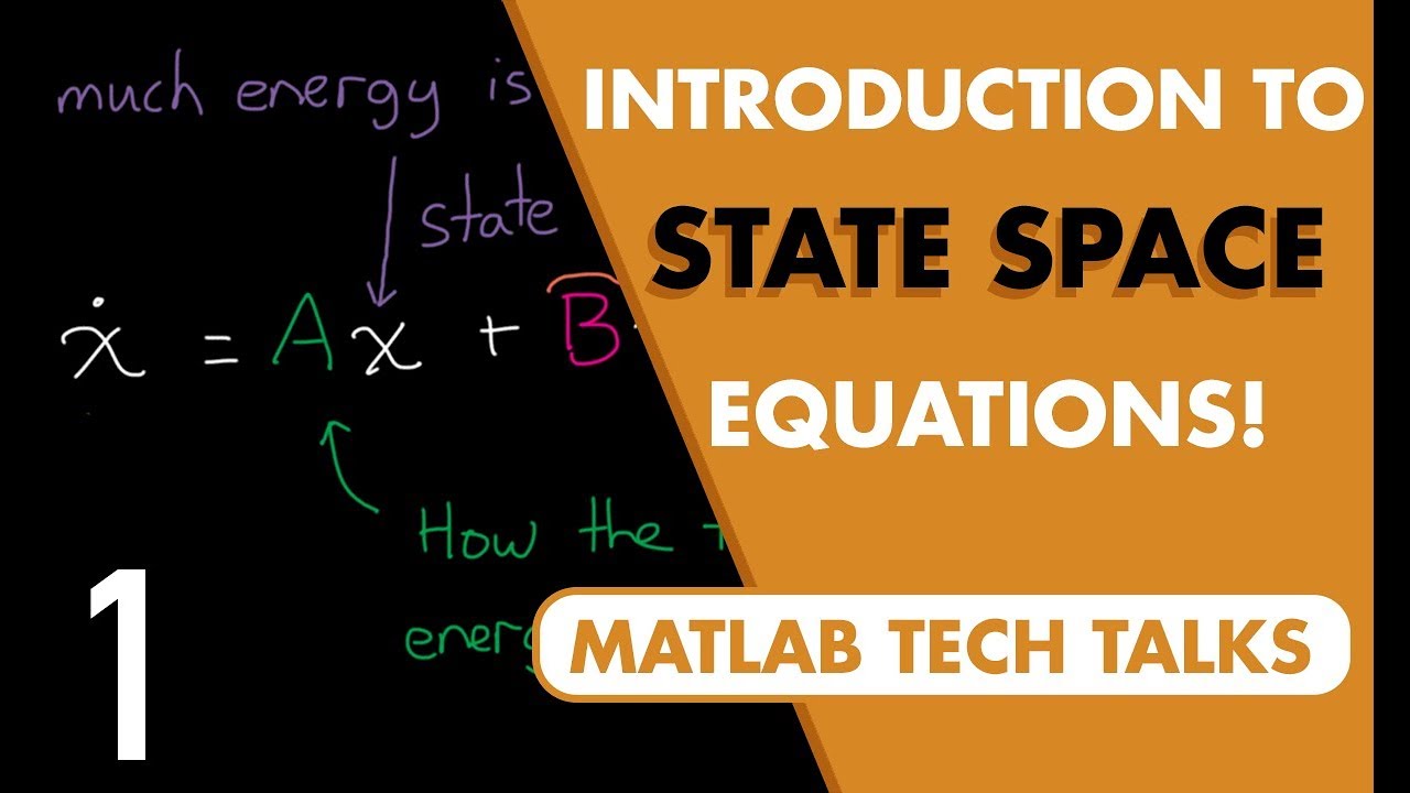


5.0 / 5 (0 votes)
