Autoregressive Models | Auto Regression | Machine Learning for Beginners | Edureka

Summary

This Edureka video introduces autoregressive models for time series forecasting, explaining the concept, types, and stationarity requirement. It covers how to select the model based on PACF plots and uses cases, including market analysis and seasonal pattern prediction, emphasizing the importance of simplicity in model selection.

Takeaways

• 📈 Auto regressive models are flexible for handling various time series patterns.
• 📚 The script introduces the concept of time series forecasting and the importance of stationarity in data for effective modeling.
• 🔢 Time series data is a sequence of data points collected at regular time intervals, such as years, months, or minutes.
• 📉 Forecasting uses historical data to predict future trends, with notations like \( y_t \), \( \phi \), \( c \), and \( \eta \) representing different elements in the time series.
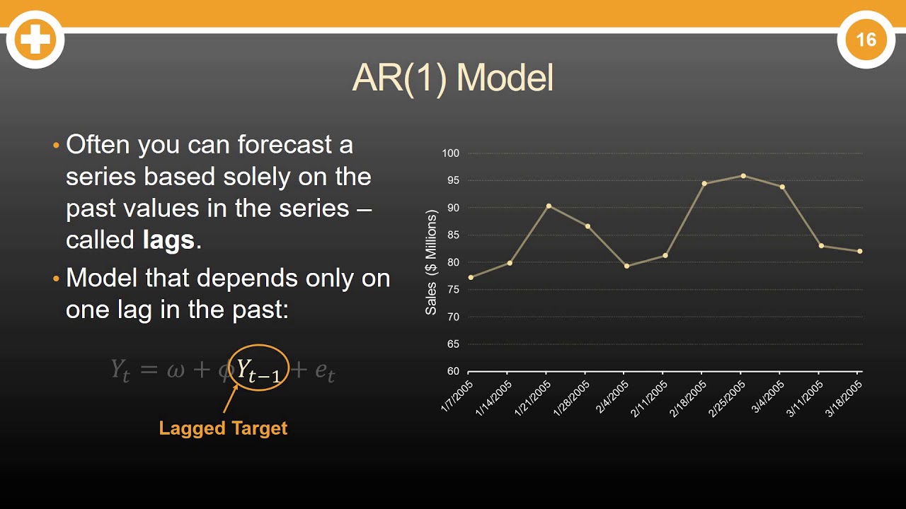
• 🔄 Auto regression is a self-referential prediction method that uses only historical data of the same variable to make predictions.
• 🚫 A key constraint for using auto regression is that the time series data must be stationary, meaning its statistical properties remain constant over time.
• 📊 Different types of autoregressive models (AR1, AR2, etc.) are determined by the number of previous time steps considered in the prediction.
• 📝 To select the appropriate autoregressive model, the script suggests using a PACF (Partial Autocorrelation Function) plot to identify significant lag values.
• 📉 The PACF plot helps in determining the partial correlation between a given time point and its lags, aiding in the selection of model parameters.
• 💡 Auto regression has various use cases, including detecting lack of randomness in data, predicting future changes, and analyzing market trends like the stock market.
• 📚 The video concludes by encouraging viewers to engage with the content, ask questions, and explore more educational material on the Edureka channel.

Q & A

What is the main focus of the video on auto regressive models?

The video focuses on explaining auto regressive models, starting with basic concepts like time series and forecasting, moving on to defining auto regression and stationarity, discussing different types of autoregressive models, how to select the appropriate model, and concluding with various use cases of AR models.

What is a time series in the context of mathematics?

A time series is a sequence of data points recorded at successive, equally spaced points in time. It represents discrete time data and can be measured in various intervals such as years, months, hours, or minutes.

How does forecasting relate to time series data?

Forecasting is a technique that utilizes historical time series data as inputs to make informed predictions about future trends. It helps in determining the direction of future movements based on past patterns.

What are the common notations used in time series data?

Common notations include 't' for the time index, 'y_t' for the value of the series at time 't', 'φ' (phi) for the coefficient of each value of 'y_t', 'c' for the constant term or bias of the model, and 'η' (eta) for the error in the forecast at time 't'.

What is meant by auto regression in the context of time series models?

Auto regression refers to a time series model that uses previous time steps' observations as inputs to predict the same characteristic at the next time step. It is based on the concept of predicting a numeric value based on its own historical data.

Why is stationarity important for using auto regressive models?

Stationarity is important because it ensures that the statistical properties of the time series data, such as mean and variance, remain constant over time. This allows for more accurate and reliable predictions using auto regressive models.

What does the term 'AR' stand for in the context of time series models?

In the context of time series models, 'AR' stands for AutoRegressive, which is a model that uses past values of a time series to predict future values.

How do you determine the number of lag values to consider in an autoregressive model?

The number of lag values to consider can be determined using a PACF (Partial AutoCorrelation Function) plot. It helps identify the significant lags by looking at the points where the PACF values fall below a certain threshold, typically a magnitude of 0.05.

What is the purpose of the constant term 'c' in an autoregressive model?

The constant term 'c' in an autoregressive model serves as the bias or the baseline value around which the predictions are made, adjusting the forecast according to the historical data's average level.

Can you provide an example of a use case for autoregressive models?

Autoregressive models are used in various fields such as predicting stock market trends, analyzing recurring or seasonal patterns in data, and detecting lack of randomness in data sequences.

Outlines

00:00

📈 Introduction to Autoregressive Models

This paragraph introduces the concept of autoregressive models in the context of time series forecasting. Kavya from Edureka explains the agenda of the video, which includes an overview of time series, the definition of auto regression and stationarity, the types of autoregressive models, how to select the appropriate model, and their use cases. The importance of stationarity for time series data is emphasized, and the basic notation used in time series analysis is defined. Autoregression is described as a model that uses previous observations to predict future values, with a simple regression equation provided as an example.

05:00

🔍 Choosing the Right Autoregressive Model

The second paragraph delves into the specifics of selecting the right autoregressive model by considering the number of lag values to include. It explains that a simple model with the least number of parameters is preferred, and introduces the Partial Autocorrelation Function (PACF) plot as a tool for determining significant lag values. The process of creating a derived chart for profit data and using the PACF plot to identify relevant lags is illustrated with an example. The paragraph concludes with examples of use cases for autoregression, such as detecting lack of randomness in data, predicting future changes, market analysis, and forecasting seasonal patterns.

Keywords

💡Time Series

A time series is a sequence of data points measured at successive points in time, typically at uniform intervals. In the video, time series refers to the structured data set that is used for forecasting future values, such as predicting profits over years or analyzing weather patterns. The concept is central to understanding how auto-regressive models function, as they rely on past values within a time series to make predictions.

💡Forecasting

Forecasting is the process of making predictions about future trends based on historical data. In the context of the video, forecasting is a key application of time series analysis, where the goal is to predict future values using models like autoregression. This is essential for planning and decision-making in various fields, such as finance and weather prediction.

💡Autoregression

Autoregression is a type of statistical model used in time series analysis where the current value of a series is predicted based on its past values. The video emphasizes that autoregression involves using previous data points from the same series to forecast future values, making it a powerful tool for time series forecasting. The term combines 'auto,' meaning 'self,' and 'regression,' which refers to predicting a numeric value.

💡Stationarity

Stationarity refers to a characteristic of a time series where its statistical properties, such as mean and variance, remain constant over time. In the video, stationarity is a necessary condition for applying autoregressive models, as non-stationary data can lead to unreliable predictions. The video explains how to identify stationary data by checking for consistent patterns over time without trends or seasonal effects.

💡AR Model

An AR (Autoregressive) model is a type of time series model that uses its own previous values to predict future values. The video discusses different types of AR models, such as AR(1) and AR(2), which differ based on how many past values are used in the prediction. The choice of the AR model depends on the data and the desired simplicity of the model.

💡Lag

Lag refers to the delay between a current data point and a previous one within a time series. In autoregressive models, lag values are the previous data points used to predict the current value. The video explains that choosing the appropriate lag values is crucial for building an effective AR model, as it determines how much past information is considered in the forecast.

💡PACF Plot

A PACF (Partial Autocorrelation Function) plot is a graphical tool used to identify the significant lags in a time series for building an AR model. The video describes how PACF plots help in determining which past values (lags) have the strongest relationship with the current value, guiding the selection of the most important lags to include in the model.

💡Coefficient (Phi)

The coefficient, denoted by the Greek letter phi (φ), represents the weight or impact of a past value (lag) on the current value in an autoregressive model. The video explains that each lag in an AR model has a corresponding coefficient that multiplies the lagged value, influencing the final prediction. These coefficients are crucial for understanding how much past data influences future outcomes.

💡Error Term (Eta)

The error term, denoted by the Greek letter eta (η), represents the difference between the actual value and the predicted value in an autoregressive model. The video highlights that every AR model includes an error term, which accounts for the unpredictable components of the data that are not captured by the model. This term is essential for assessing the accuracy and reliability of the model's predictions.

💡Use Cases of Autoregression

The video outlines various use cases of autoregression, emphasizing its application in predicting future trends, analyzing market data, and identifying patterns in time series. Examples include forecasting stock market trends and detecting seasonal patterns in sales data. Understanding these use cases helps viewers grasp the practical significance of autoregressive models in real-world scenarios.

Highlights

Auto regressive models are introduced as flexible for handling various time series patterns.

Agenda includes time series and forecasting, auto regression, stationarity, types of autoregressive models, model selection, and use cases of AR.

Time series is defined as a sequence of discrete time data taken at equally spaced points in time.

Forecasting is explained as using historical data to make predictive estimates for future trends.

Time series data notations are introduced, including index 't', series values 'y_t', coefficients 'φ', constant 'c', and forecast error 'η'.

Auto regression is defined as a time series model using previous time steps' observations to predict future characteristics.

Stationarity in time series is the condition where statistical properties remain constant over time without trends or changing variance.

Different types of autoregressive models (AR1, AR2, etc.) are based on the number of previous values considered for prediction.

The simplest model with the least number of parameters is preferred in auto regression.

PACF plot is used to determine the lag values to consider in the model, based on partial autocorrelation.

A practical example of using PACF plot for selecting significant lags in a profit time series is provided.

Auto regression can identify lack of randomness in data through its auto correlation-based model.

Primary use case of auto regression is predicting future changes using time series indexing.

Auto regression is commonly used in market analysis, such as the stock market, to forecast trends.

The model can also forecast recurring or seasonal patterns in data.

The video concludes with an invitation for viewers to subscribe, like, and comment for further learning.

Transcripts

[Music]

auto regressive models are remarkably

flexible at handling a wide range of

different time series patterns hi guys

this is kavya from edureka welcome to

this video on auto regressive models at

first let's have a look at the agenda

we'll start with time series and

forecasting and then we'll see what is

auto regression and what is stationarity

we'll have a look at the types of

autoregressive models and followed by

how to pick the autoregressive model

we'll conclude the session with the use

cases of ar

but before we get started make sure you

subscribe to edirect youtube channel and

hit the bell icon to never miss an

update also if you are interested in

online training certification do check

out the link given in the description

now let's go ahead and have a brief

introduction to time series and

forecasting in mathematics a time series

is a sequence taken at a successively

equally spaced points in time

thus it is a sequence of discrete time

data

the time can be of any order such as in

terms of years months hours or minutes

for example analyzing profits in a

company over many years would be an

example of time series or checking the

weather at different time stamps can

also be a time series however checking

the temperature over different matrix

such as city or latitude will not be an

example of time series so using suitable

time series forecasts can be made

forecasting is a technique that uses

historical data as inputs to make

informed estimates that are predictive

in determining the direction of future

trends

there are various notations used in time

series data the alphabet t taking

numeric values such as 1 2 3 etc is the

index denoting the particular time

period

y t would be the series of n values

corresponding to each time index d the

greek alphabet phi denotes the

coefficient for each value of y t

c is a constant term denoting the bias

of the model and eta denotes the error

in forecast in time t given the actual

value y t minus the forecasted value f d

having familiarity with time series and

the notations now let's have a look at

what auto regression is

the term auto regression is composed of

two terms auto and regression

the term regression refers to the

prediction of some numeric value this

value can be of any scale and still be

regressive

and auto here means self that is

prediction of numeric value based on its

own previous cells

no other factors are taken into

consideration except for its own

historical data consider this example

here the price of an object is

determined based on the date the

predictions are only based on its own

older values thus we can say that auto

regression is a time series model that

uses observations from previous time

steps as inputs to predict the same

characteristics at the next time step

to calculate the value at time step t

for value y the regression equation

looks like this where y d is the value

at time t

c is the constant phi is the coefficient

to each of the previous time stem values

and eta is the error term of the

equation a constraint to using

autoregression is that the time series

data needs to be stationary so now let's

have a look at what do we mean by

stationarity time series data is said to

be stationary if the statistical

properties do not change over time

it is supposed to show an inclining or

declining overall trend so the mean and

variance should remain constant over

different slices in the data

also a time series with seasonal

patterns with no clear trend is not

stationary

for example this data depicts incline in

some months and decline in some others

forming a seasonal pattern hence it is

not stationary however this data is

showing a clear inclining trend so it is

an example of stationary data so guys

when we know that the data is stationary

we can proceed with auto regression now

let's have a look at the various kinds

of autoregressive models

when i talk about the types of

autoregressive models i mean the number

of previous values to take into account

let's see in this example we have data

till 2020 for profit and we want to find

the profit for the coming year that is

2021. the type of ar model will

determine which of the date from the

previous years we will take into

consideration

ar1 will only take one previous year's

data point into consideration the

equation shows that to determine yt we

are only taking the value of y of t

minus 1 along with its coefficient phi

constant c and error term eta similarly

ar2 takes both the data of t minus 1 and

t minus 2 to predict y t

note that in the equation there's always

one constant and one error term but the

number of coefficients of older values

depends on the type of autoregressive

model we take

the number of previous values is not

limited to one or two it can be any p

values taken into consideration

accordingly the equation will contain p

coefficients 2.

now that we know about the kinds of

autoregressive models let's find out how

to pick the number of lag values to

consider

you might think that it's obvious to

consider all the previous data points to

build a model however the rule of auto

regression is to make the simplest model

with least number of parameters

to determine which lag values to take we

can consider something known as a pacf

plot

pacf stands for partial autocorrelation

function as explanatory with the name it

determines the partial correlation

between a given point and its lag or

previous value we can only take into

account those parameters for which the

lag is higher than the threshold value

consider this plot

the data points corresponding to each

year looks like this we have profit for

each year

from this data we need to make a derived

chart where we will take the difference

in profit between that year and two

years before so lag will be equal to 2

and we will find the value of y of t

minus y of t minus 2 thus lag of 2020

will be profit of 2020 which is 82 minus

profit of 2018 which is 93 that is equal

to minus 11.

lag of 2018 will be profit in 2018 minus

profit in 2016 which is 93 minus 94

equals minus 1 and so on

for this data we make a pacf plot taking

threshold as magnitude of 10.

from this plot we see that the profit

lag for the years 2014 and 2018 is below

the magnitude of 10. thus we will only

take the points of yt with t equals 2012

2016 and 2020.

the equation for this function will be

the forecasted value for 2021

equals constant c plus phi into y of

2012 plus phi into y of 2016 plus phi

into y of 2020 plus the error term eta

this is the simplest equation of auto

regression to forecast the time series

taking only the significant lags

finally let's have a look at some of the

use cases of auto regression the model

of auto regression is based on auto

correlation thus auto regression can

help us find if there is a lack of

randomness in the data

secondly as we have seen the primary use

case of autoregression is to predict

future changes using time series

indexing

auto regression is also commonly used to

analyze markets such as stock market

it can also forecast any kind of

recurring or seasonal pattern in the

data

i hope you enjoyed the session thank you

for watching this video if you have any

doubts please leave a message in the

comment section happy learning

i hope you have enjoyed listening to

this video please be kind enough to like

it and you can comment any of your

doubts and queries and we will reply

them at the earliest do look out for

more videos in our playlist and

subscribe to edureka channel to learn

more happy learning

you