FEA V29: Gaussian Quadrature
Summary
TLDRThis video script delves into Gaussian quadrature, a pivotal method for numerical integration in finite element analysis. It explains how Gaussian quadrature is used to calculate the stiffness matrix by integrating over an element's volume. The script highlights the importance of the Jacobian determinant in transforming integrals from global to local coordinates. It also discusses the properties of the B matrix and the challenges of integrating ratios of polynomials. The script further illustrates how Gaussian quadrature efficiently approximates integrals of polynomial functions with fewer function evaluations, providing examples of single, double, and triple integration points for increasing accuracy. Finally, it applies Gaussian quadrature to evaluate a nodal force vector, demonstrating the trade-off between accuracy and computational efficiency.
Takeaways
- 📐 Gaussian quadrature is a method for numerical integration used in finite element analysis.
- 🌐 The isoparametric stiffness matrix is calculated by integrating over the volume of an element using B transpose times D times B.
- 🔍 The Jacobian determinant is key in transforming integrals from global to local coordinates, simplifying the process.
- 📏 The limits for the natural coordinates s and t in numerical integration typically range from -1 to 1.
- 📈 B matrices depend on nodal positions, making each element's B matrix distinct in the global system.
- 🔢 Good elements have linear terms in B and B transpose, leading to quadratic expressions when multiplied.
- 📉 Poor quality elements can result in complex ratios of polynomials for the Jacobian determinant, complicating integration.
- 📋 Gaussian quadrature is efficient for polynomial integrands, requiring fewer function evaluations for the same accuracy.
- 📊 The method involves evaluating the function at specific locations (integration points) and multiplying by interval widths for area approximation.
- 📉 Using more integration points increases accuracy but also the computational cost, as it requires more function evaluations.
- 🔧 An example demonstrates the difference between single and two-point Gaussian quadrature, with the latter providing exact results for quadratic functions.
Q & A
What is Gaussian quadrature?
-Gaussian quadrature is a method for numerical integration that is particularly efficient for polynomial integrands. It approximates the integral of a function by evaluating it at specific points (integration points) and multiplying by weights, which are determined to minimize the number of evaluations needed for a given level of accuracy.
Why is Gaussian quadrature important in finite element analysis?
-In finite element analysis, Gaussian quadrature is crucial for calculating the stiffness matrix of each element in a structure. It allows for the transformation of the integration from the global coordinate system to the natural coordinate system, simplifying the process and making it computationally efficient.
What is the significance of the Jacobian determinant in Gaussian quadrature?
-The Jacobian determinant is significant because it relates the infinitesimal areas in the global coordinate system to the natural coordinate system. It is used to transform the limits of integration from global to local coordinates, which simplifies the integration process in finite element analysis.
How does the quality of an element affect the integration process?
-The quality of an element affects the integration process because it influences the complexity of the integrand. Good quality elements have simpler integrands, often polynomials, which are easier to integrate using Gaussian quadrature. Poor quality elements may have more complex integrands, such as ratios of polynomials, which are harder to integrate.
What are the properties of the B matrices in the context of Gaussian quadrature?
-The B matrices in Gaussian quadrature depend on the nodal positions and are used to map from the natural to the global coordinate system. Each B matrix is distinct for each element because it depends on the element's nodal positions. The B matrices are defined in terms of natural coordinates s and t.
How does the number of integration points affect the accuracy of Gaussian quadrature?
-The number of integration points in Gaussian quadrature directly affects the accuracy of the numerical integration. More points generally provide higher accuracy, especially for higher-degree polynomial integrands. However, it also increases the computational cost, as more function evaluations are required.
What is the role of the integration points in Gaussian quadrature?
-Integration points in Gaussian quadrature are the specific locations at which the function is evaluated. These points are chosen to optimize the accuracy for polynomial integrands. The choice of these points, along with the interval width, determines the efficiency and accuracy of the numerical integration.
Why is it beneficial to evaluate the function at the midpoint in a single integration point scenario?
-Evaluating the function at the midpoint in a single integration point scenario is beneficial because it provides an exact result for linear integrands. This is due to the property that a linear function will average out to zero over a symmetric interval, resulting in an exact integral value.
How does the width of the rectangles in Gaussian quadrature relate to the number of integration points?
-The width of the rectangles in Gaussian quadrature changes with the number of integration points. With more points, the rectangles may have different widths, with the central rectangle often being wider to give more emphasis to the central region of the integration range, which is especially important for higher-degree polynomials.
What is the practical example given in the script for using Gaussian quadrature?
-The practical example given in the script is the evaluation of a nodal force vector in a finite element model. The script explains how Gaussian quadrature can be used to approximate the integral of a quadratic function to find the force vector, with different levels of accuracy depending on the number of integration points used.
What is the difference between one-point and two-point Gaussian quadrature integration?
-One-point Gaussian quadrature integration evaluates the function at the midpoint of the interval and is exact for linear integrands. Two-point integration evaluates the function at two specific points and is exact for cubic integrands. The two-point method is more accurate for quadratic integrands compared to the one-point method.
Outlines

Cette section est réservée aux utilisateurs payants. Améliorez votre compte pour accéder à cette section.
Améliorer maintenantMindmap

Cette section est réservée aux utilisateurs payants. Améliorez votre compte pour accéder à cette section.
Améliorer maintenantKeywords

Cette section est réservée aux utilisateurs payants. Améliorez votre compte pour accéder à cette section.
Améliorer maintenantHighlights

Cette section est réservée aux utilisateurs payants. Améliorez votre compte pour accéder à cette section.
Améliorer maintenantTranscripts

Cette section est réservée aux utilisateurs payants. Améliorez votre compte pour accéder à cette section.
Améliorer maintenant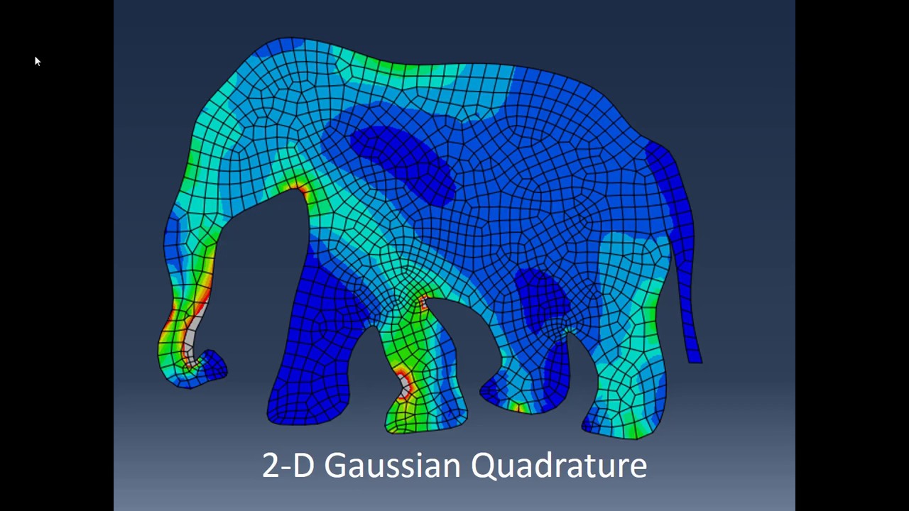


5.0 / 5 (0 votes)
