Master Data Analysis on Excel in Just 10 Minutes
Summary
TLDREste vídeo enseña los fundamentos del análisis de datos dividiéndolo en cuatro áreas clave: transformación de datos, creación de estadísticas descriptivas, análisis de datos y creación de un informe para visualizar los resultados. Se muestra cómo limpiar datos en Excel, usar fórmulas para redondear y agregar columnas, y cómo detectar duplicados. Además, se explica cómo realizar estadísticas descriptivas y análisis de datos con herramientas como el análisis de datos y tablas dinámicas, y cómo generar informes interactivos con validación de datos y formateo condicional.
Takeaways
- 😀 Aprenderás los fundamentos del análisis de datos divididos en cuatro áreas principales: transformación de datos, creación de estadísticas descriptivas, análisis de datos y creación de un informe para visualizar los resultados.
- 🧼 El primer paso es transformar y limpiar los datos utilizando herramientas como Excel y técnicas de limpieza como la función TRIM para eliminar espacios innecesarios.
- 📈 Se utiliza la función ROUNDUP para redondear los valores decimales a números enteros, lo cual es crucial cuando los datos representan cantidades físicas como comida.
- 🗺️ Añadir información relevante como los países asociados a las ciudades en los datos puede ofrecer un contexto más completo y ser útil para el análisis.
- 🔍 Comprobar y eliminar duplicados en los datos es esencial para garantizar la precisión y la calidad del análisis.
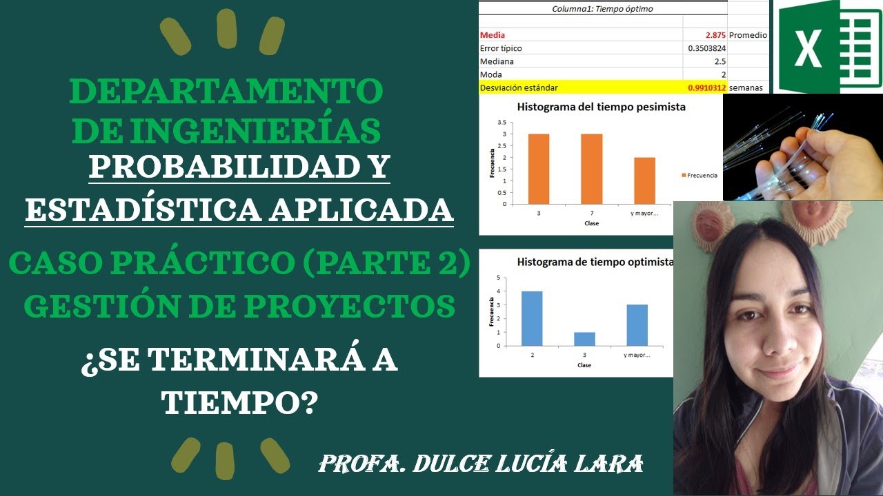
- 📊 La creación de estadísticas descriptivas, como el promedio, mínimo, máximo y moda, ayuda a entender mejor los datos utilizando herramientas como el análisis de datos en Excel.
- 📊 La utilización de gráficos de caja y bigotes (box and whisker) permite identificar outliers y comprender la distribución de los datos.
- 📊 Para una mayor profundidad en el análisis, es posible desglosar los datos por categorías específicas, como el nombre del gerente, para identificar tendencias o problemas.
- 📊 El análisis de datos también incluye responder a preguntas específicas, como qué producto es el más vendido, cuál es el ingreso total y cómo se distribuye el ingreso por método de pago.
- 📊 La creación de tablas dinámicas como las tablas dinámicas de Excel permite desglosar y analizar datos de manera eficiente y efectiva.
- 📊 La finalización del análisis con la creación de un informe que incluye validación de datos, fórmulas y formato condicional para presentar los resultados de manera clara y accionable.
Q & A
¿Qué áreas principales se abordan en el video sobre análisis de datos?
-El video se divide en cuatro áreas principales: transformación de datos, creación de estadísticas descriptivas, análisis de datos y creación de un informe para visualizar los resultados.
¿Cómo se transforma y limpia el conjunto de datos en Excel?
-Para transformar y limpiar los datos en Excel, se convierte el conjunto de datos en una tabla, se eliminan espacios extra en la columna del gerente usando la función TRIM, se redondean los números decimales en la columna de cantidad al número entero más cercano usando la función ROUNDUP y se eliminan duplicados.
¿Qué función de Excel se utiliza para eliminar los espacios innecesarios en una columna?
-Para eliminar los espacios innecesarios en una columna, se utiliza la función TRIM.
¿Cómo se redondea un número a un entero completo en Excel?
-Para redondear un número a un entero completo en Excel, se utiliza la función ROUNDUP, especificando el número y el número de dígitos, que en este caso es cero.
¿Cómo se pueden agregar países a una lista de ciudades en Excel?
-Para agregar países a una lista de ciudades en Excel, se utiliza la función de tipos de datos geográficos, donde se puede añadir una columna que asocie un país o región con cada ciudad.
¿Qué herramienta en Excel permite realizar análisis estadísticos descriptivos rápidamente?
-La herramienta de análisis de datos en Excel permite realizar análisis estadísticos descriptivos rápidamente, proporcionando información como la media, mediana, moda, mínimo, máximo, suma y más.
¿Cómo se crea un gráfico de caja y bigotes en Excel para identificar outliers en los precios?
-Para crear un gráfico de caja y bigotes en Excel, se seleccionan los precios, se utiliza la opción de gráfico de caja y bigotes y se personaliza para mostrar la distribución de datos, incluyendo los outliers.
¿Cómo se determina el producto más vendido y el análisis de la estructura de ingresos por método de pago en el video?
-Para determinar el producto más vendido y el análisis de la estructura de ingresos por método de pago, se utiliza una tabla dinámica, donde se calcula el ingreso total multiplicando el precio por la cantidad y se muestran los resultados como porcentajes del total general.
¿Qué es el certificado de análisis de datos de Google y cómo se relaciona con el contenido del video?
-El certificado de análisis de datos de Google es un programa diseñado para enseñar habilidades laborales para cualquier rol de análisis de datos. Se menciona en el video como una opción para aquellos que quieran profundizar en el aprendizaje de habilidades de análisis de datos.
¿Cómo se crea un informe final en Excel que incluya validación de datos y formateo condicional?
-Para crear un informe final en Excel, se utiliza la validación de datos para permitir la selección de un gerente, lo que provoca que otros datos como país y ciudad se actualicen dinámicamente usando la función VLOOKUP. Además, se aplican barras de datos usando el formato condicional para representar visualmente la información.
¿Cómo se activa el Analysis Toolpack en Excel si no está disponible inicialmente?
-Para activar el Analysis Toolpack en Excel, se va a Archivo > Opciones > Complementos, se selecciona el Analysis Toolpack y se hace clic en Ir y luego en OK.
Outlines
📊 Análisis de datos básico: Transformación y limpieza de datos
Este primer párrafo explica cómo iniciar el análisis de datos con la transformación y limpieza de datos. Se menciona la necesidad de limpiar los datos para su análisis y se presenta un ejemplo práctico utilizando un archivo de Excel para un cajero automático. Se detalla cómo transformar un conjunto de datos en una tabla, cómo limpiar espacios en columnas específicas utilizando la función TRIM y cómo cambiar los nombres de las columnas. Además, se aborda la problemática de los decimales en la cantidad de productos y cómo redondear estos valores al número entero utilizando la función ROUNDUP. También se discute la adición de información relevante como los países asociados a las ciudades y cómo eliminar duplicados en los datos.
📈 Análisis descriptivo y visualización de datos
El segundo párrafo se enfoca en el análisis descriptivo de los datos y la creación de informes visuales. Se describe cómo activar herramientas de análisis de datos en Excel y cómo generar estadísticas descriptivas para los precios y las cantidades de productos. Se explica el uso de la herramienta de análisis de datos para obtener la media, mediana, moda, mínimo, máximo y otros datos relevantes. Además, se menciona cómo identificar outliers utilizando un gráfico de caja y bigote y cómo profundizar en el análisis al desglosar los datos por nombre de gerente. Se sugiere la importancia de la visualización de datos y cómo se puede mejorar la presentación de los datos en un informe final.
💼 Análisis de datos avanzado y creación de informes
El tercer párrafo trata sobre el análisis de datos avanzado y cómo presentar los resultados en un informe. Se describe cómo calcular el ingreso total y el desglose por método de pago utilizando tablas dinámicas y cómo determinar el producto más vendido. Se explica cómo crear un informe final que incluya validación de datos, fórmulas de búsqueda y barras de datos condicionadas para presentar de manera clara y efectiva los resultados del análisis. Se enfatiza la importancia de la presentación y cómo se puede personalizar el informe para diferentes gerentes y productos.
Mindmap
Keywords
💡Análisis de datos
💡Transformación de datos
💡Estadísticas descriptivas
💡Visualización
💡Limpieza de datos
💡Formularios de Excel
💡Redondeo
💡Duplicados
💡Análisis de caja y bigotes
💡Pivot table
💡Validación de datos
Highlights
Introduction to the fundamentals of data analysis
Data transformation and cleaning
Creating descriptive statistics for better understanding
Data analysis techniques
Visualization of findings through report creation
Sponsor mention: Coursera
Transforming data by converting it into a table
Cleaning up data by removing extra spaces
Rounding up quantities to whole numbers
Adding country information to city data
Removing duplicates from the dataset
Introduction to Google's data analytics professional certificate
Calculating descriptive statistics using Excel
Using Data Analysis tool for quick statistics
Creating a box and whisker chart to identify outliers
Analyzing data by manager to identify potential data entry issues
Calculating revenue by multiplying price and quantity
Using pivot tables for data analysis
Determining the best selling product
Calculating total revenue
Revenue breakdown by payment method
Creating a dynamic report with data validation
Using conditional formatting for data bars
Transcripts
in this video you're going to learn all the fundamentals of data analysis and we'll break
this down into four main areas first we're going to be looking at transforming the data
so cleaning it up secondly we're going to be looking at creating descriptive statistics to
understanding better third we're going to be looking at data analysis and finally we'll get
into creating a report to visualize our findings so let's get into it and thank you to Coursera
for sponsoring this video more on them later the first step here is to transform the data and for
this here's the Excel file that we'll be working with which you can download for free in the video
description so as you can see this is going to be for a fast food chain you can see the types
of products here and the first step is simply to clean this up but for that we're going to
go to control T So to change this into a table so change the data set into a table then we'll
head on OK from here for the cleanup part you can see that under the manager column we seem to have
some very odd spacing here so let's go ahead and clean that up here we're going to go to equals
trim hit the top key and this formula is going to remove these old spaces I'm going to hit enter
there you can see that's going to Auto populate for all of these we'll change this name to manager
and then for all of these that are currently linked to this column over
here we're going to paste them as values so we're going to go Ctrl shift down
Ctrl C and then we're gonna paste this as a value so alt h v v is a shortcut for that and now that
means that we can go ahead and remove this column by hitting Ctrl minus there you go then under
quantity you might notice that we've got these decimals which don't make too much sense you can't
really have half a burger and so for this we're basically gonna have to round up to a whole number
for that we're going to use the Roundup formula so equals round up hit the top key there the number
is this one comma and the number of digits for us is going to be zero because we want the full
number close those brackets and hit enter so this is going to be our quantity now hit enter there
and we basically wanna Ctrl shift down Ctrl C and then paste as values so alt h v v v again
there you go so now we can remove this column here so we're going to select it and control minus
then you'll notice that under City here we have the city names but we don't necessarily have
the countries that would be a nice thing to add so for this we can actually head over to the data tab
and go under data types you'll find geography here so just click on that
once you start to see that icon it means that it's loaded up what you want to do here is
hit over to this icon to the side under add column and we basically want to add a country
or a region associated with that City and you can see that we have the corresponding country
for each City if you want to move this city column next to the country you can actually
go ahead and select it up top and we start to see these arrows when you hover over it just
press the shift key and then just drag it across like so that should allow you to move everything
one final thing we haven't done here is test if there's any duplicates so for this we can
simply go under data again and we're just going to remove duplicates by going to this icon over here
so we'll click on that and it's going to be for that whole table and we'll simply hit on OK
and you can see here that we get a notification saying that five duplicate values were found and
removed so we'll hit on OK there and speaking of data analysis if this is something that
you want to learn more about you can check out Google's data analytics professional certificate
it's designed to teach you job ready skills for any data analytics role so you can learn
all the skills required in less than six months the program currently has well over 1 million
students in a 4.8 star rating now if you're wondering if you need any prior experience no
there's no prior experience required and it's all fully self-paced in the program you learn
key analytical skills including data cleaning analysis and visualization using some of the
most common industry tools such as spreadsheets SQL or R programming upon completion you'll
receive a Google professional certification which you'll be able to share on your CV and Linkedin
so if you're interested sign up for a seven day free trial Now using the link in the description
below alright back to the video great now that we've done step one and step two it's
all about the descriptive statistics so really seeing things like what's the average price what
about the minimum the maximum and so on so for this let's hop over to the side and you could
try to find for the price and for the quantity say the average going one by one so type the average
formula then doing the same thing with the minimum the maximum so on but there is a much faster way
that's actually using a tool called Data analysis for that we're gonna have to activate it it should
be over here to the side under the data ribbon if you don't have it like me we can go ahead
and activate it so we'll head over to file go over to the bottom where it says options
from here we're gonna go into add-ins and we want to click on the analysis toolpack here and hit on
go from here we want to select analysis toolpack like I said and we'll hit OK now you can see that
we have this data analysis option under the data ribbon so that's the one that we want to select
from here we want the descriptive statistics and we'll hit on OK there
and the input range is going to be all of our prices so we'll go Ctrl shift down there
and then we want it to be a summary statistics and where do we want this let's say we want an output
range which is going to be up over here so right next to the table let's say we put it here to the
side there we're just going to hit on OK and now you can see that for the price which is what we've
selected we've gotten everything from the mean the median mode minimum maximum sum and a bunch
of other useful information let me repeat that same process for the quantity awesome now we've
got the breakdown by price and by quantity as well but one thing that this doesn't quite account for
is the fact that there could be outliers in our price so for that we can go ahead down over here
we're gonna basically create a new chart which is going to be a box and whisker so let's first
select all of the prices so Ctrl shift down and down over here you're gonna find this icon
click on that and we want a box and whisker basically this one over here and don't worry
if you can't interpret it we'll look at it just in a second let me move that all the way up
so once we have it in here this is basically telling us a few different things so first
these top and bottom lines are telling us the maximums so the Max and the Min if you
will and then in here this box represents the first and the third quartile and then you can
see that we've got that X which is the average then we've got a line which is going to be the
median and finally we've got these dots over here which represent all of our outliers in our price
now if we want to dig a bit further into this it would be nice to see the x-axis maybe we can
put something like the manager's name to see where exactly this is coming from maybe it's one manager
that might be reporting the data wrong so we'll go to right click for that go under select data
edit the horizontal category access label here and what we're going to do is put the
managers so we're going to select all of these Ctrl shift down and hit on OK
and hit on OK again now if we go all the way back up you can see what that breakdown looks like
by manager and it seems to be that all of these outliers are accumulated with Joel maybe we should
have a word with him now moving on to step 3 which is data analysis so over here you can see that
we've got three different questions that we want to solve which is what is our best selling product
what is our total revenue and that's what's our Revenue breakdown by payment method so if we go
back to the table here you notice that we don't actually have a column for Revenue so that's one
that we're going to have to calculate simply by multiplying the price and the quantity so
we'll do that over here let me add an extra column there and let's call this something like Revenue
and the formula for it is going to be equals the quantity multiplied by the price and we'll just
hit enter there that should be calculated for us and then we'll go up over here again and for all
of this analysis we can actually do most of it with a pivot table so we'll head over to insert
pivot table the table or range we're interested in is all of this range so once we select one of the
cells we can just go to control a that's going to select all of them and we want this in a location
in an existing worksheet which we already selected so we'll hit OK great from here we can start doing
all the breakdown so what's our best selling product so let's do this by quantity we're going
to select the products as the rows just hover that over and then we're gonna check the quantity over
here as the values great now we have all of that breakdown if we want to sort it from highest to
lowest we can go to right click and go to sort and we'll sort largest to smallest and now you
can see that beverages is our largest at 35 000. then secondly we've got what is our total revenue
for this one we're simply going to have to select the revenue so first we'll remove these let's take
this out and we'll take this out as well and we just have to select the revenue and put it
under values that should give us the sum of total revenue which seems to be 812 000. and finally our
Revenue breakdown by payment method so for that we're gonna get all of the payment methods and
put those under the rosie like so but to see the breakdown better it probably makes more sense as
a percentage so what we can actually do is go to right click and from here go to summarize show
values ask sorry and we're going to show them as a percentage of the grand total now you can see that
full breakdown and it seems like credit cards are the most dominant here now that you've seen how to
do some of the data analysis let me show you what a final report might look like this one here is
fairly simplified so you can see that we've got this drop down which is using data validation
to select the manager and everything dynamically changes so if I select dwell I'm able to see which
country and city is from using the X lookup and then just below that using the sum ifs I'm able
to derive his particular revenue for fries and the other products as well as his total revenue
and these data bars over here are done using the conditional formatting if you're unsure
how to do this type of formulas you can check out this video over here or this link over here
to take our Excel codes hit the like and that subscribe and I'll catch you in the next one
Ver Más Videos Relacionados
5.0 / 5 (0 votes)