The spherical harmonics

Summary

In this video, Professor Erin Das explores spherical harmonics, essential eigenfunctions in quantum mechanics, particularly relevant to the hydrogen atom. The discussion covers their mathematical forms, visualization techniques, and their role in describing orbital angular momentum. Using visual representations on the unit sphere, the video explains the angular dependence of spherical harmonics and how they vary with quantum numbers l and m. The content is supported by Python code available through a linked Jupyter notebook, encouraging viewers to interact with and generate their own visualizations. This video is ideal for anyone interested in the mathematical beauty and application of spherical harmonics in quantum systems.

Takeaways

• 📚 Spherical harmonics are the eigenfunctions of orbital angular momentum in quantum mechanics, crucial in many problems, especially in the hydrogen atom.
• 🔢 These harmonics depend on two quantum numbers: l (angular momentum) and m (magnetic quantum number).
• 📈 Spherical harmonics are often visualized on the unit sphere, where positive values are red, negative values are blue, and zero values are white.
• 🧮 The Y00 spherical harmonic is a constant function, representing a uniform red sphere, while Ylm functions show more complex patterns depending on l and m.
• 🎨 The visualization of spherical harmonics helps in understanding their angular dependence, with each harmonic represented by color-coded spheres based on their values.
• 🔄 The values of spherical harmonics can change with the angles θ and φ, producing varying patterns across different harmonics as l and m increase.
• 💻 The script refers to a linked Jupyter notebook containing Python code that can generate spherical harmonics, allowing viewers to visualize them themselves.
• 🔬 Spherical harmonics play a central role in quantum mechanics, especially in understanding the angular part of wavefunctions in the hydrogen atom.
• 🔍 The script also explains how spherical harmonics are related to associated Legendre polynomials and their use in different mathematical forms.
• 🔧 An alternative way to visualize spherical harmonics is by plotting the magnitude of the function, which produces different, often used, visual representations.

Q & A

What are spherical harmonics and why are they important in quantum mechanics?

Spherical harmonics are the eigenfunctions of orbital angular momentum in quantum mechanics. They are important because they describe the angular part of wavefunctions in systems such as the hydrogen atom, making them crucial for solving problems involving spherical symmetry.

What is the general form of a spherical harmonic function?

The general form of a spherical harmonic function \( Y_{l}^{m}(θ, φ) \) consists of a pre-factor, a phase factor, and a term involving associated Legendre polynomials, depending on the angular variables \( θ \) (colatitude) and \( φ \) (azimuthal angle).

What are the quantum numbers associated with spherical harmonics?

Spherical harmonics are labeled by two quantum numbers: \( l \), which is associated with the magnitude of orbital angular momentum, and \( m \), which describes the z-component of angular momentum. The values of \( l \) are non-negative integers, and for a given \( l \), \( m \) ranges from \( -l \) to \( l \).

How do spherical harmonics relate to the hydrogen atom?

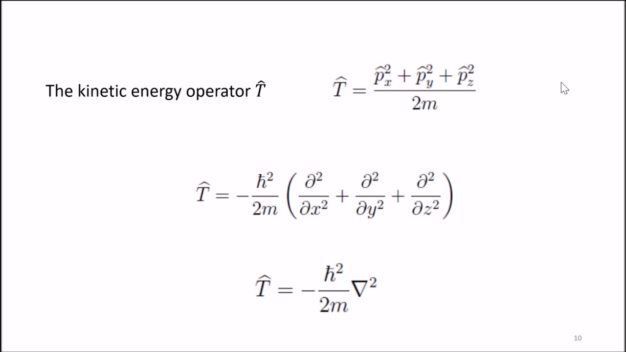
In the hydrogen atom, spherical harmonics describe the angular part of the electron's wavefunction. This is due to the spherical symmetry of the atom, making spherical harmonics essential for solving the Schrödinger equation in spherical coordinates.

What do the colors in spherical harmonic visualizations represent?

In spherical harmonic visualizations, colors represent the value of the function at each angular position on the unit sphere. Red indicates positive values, blue indicates negative values, and white corresponds to zero. These visualizations help show the angular dependence of the function.

How are spherical coordinates used in the context of spherical harmonics?

Spherical coordinates are used to describe the position of a point in space using three numbers: \( r \) (distance from the origin), \( θ \) (angle from the z-axis), and \( φ \) (angle in the horizontal plane from the x-axis). Spherical harmonics depend only on \( θ \) and \( φ \), making them ideal for problems with spherical symmetry.

What are associated Legendre polynomials and their role in spherical harmonics?

Associated Legendre polynomials, denoted as \( P_{l}^{m}(\cos θ) \), appear in the mathematical expression of spherical harmonics. They define the angular dependence of spherical harmonics in terms of the colatitude angle \( θ \).

What does the spherical harmonic \( Y_{0}^{0} \) look like?

The spherical harmonic \( Y_{0}^{0} \) is a constant and has no angular dependence. It is represented by a uniformly red sphere because the function has the same value at all points on the unit sphere, corresponding to a value of \( 1 / \sqrt{4π} \).

How do the real and imaginary parts of spherical harmonics differ in their visual representation?

The real and imaginary parts of spherical harmonics can be represented separately. For example, for \( Y_{1}^{-1} \), the real part exhibits a cosine dependence, while the imaginary part exhibits a sine dependence. These two parts are 90 degrees out of phase and show different patterns in the color plot.

What are the common methods for visualizing spherical harmonics, and how do they differ?

There are two common methods for visualizing spherical harmonics. One plots the function on a unit sphere, using colors to represent the value at different angles. Another method uses the magnitude of the function to define a radial distance, effectively stretching the surface based on the function's value. Both methods highlight different aspects of the function's angular dependence.

Outlines

00:00

🔬 Introduction to Spherical Harmonics in Quantum Mechanics

Professor Erin Das introduces spherical harmonics, which are eigenfunctions of orbital angular momentum in quantum mechanics. The discussion centers on their role, particularly in the hydrogen atom. The video will explore the mathematical forms of spherical harmonics, visualize them, and provide Python code to generate these plots.

05:01

🌈 Visualizing Spherical Harmonics on the Unit Sphere

The visualization of spherical harmonics is explained, where the color represents function values on the unit sphere. Red indicates large positive values, blue indicates large negative values, and white represents zero. The angular coordinates, theta and phi, help describe points on the sphere, and rotation helps in better understanding these visualizations.

10:02

📐 Real and Imaginary Parts of Spherical Harmonics

The focus shifts to the real and imaginary parts of spherical harmonics, starting with the case of l=1, m=-1. The behavior of the spherical harmonics is broken down by analyzing how the cosine and sine functions change across different angles, giving insight into the patterns of positive and negative values across the surface.

15:03

🎨 Exploring Various Quantum States: L=1 and Beyond

Different spherical harmonics for quantum states with l=1 and varying m are explored, including their mathematical derivation and visual representation. The constant nature of some functions across specific angles and their color-coded depiction is discussed. This provides deeper insights into how different quantum states manifest geometrically.

20:04

🔢 Understanding Higher-Order Spherical Harmonics

The video explores spherical harmonics with l=2, presenting five possible states (m = -2 to 2) and their corresponding mathematical and visual representations. The complex patterns of these harmonics are visualized in both real and imaginary parts, showcasing their beauty and symmetry in quantum mechanical systems.

💻 Generate Your Own Spherical Harmonics with Python

A detailed comparison is provided between traditional spherical harmonics plots and an alternative approach where the magnitude of the function defines a radial distance. The rotation of these plots helps viewers understand the full angular dependence. The video concludes by encouraging viewers to use Python code to create their own spherical harmonics.

Keywords

💡spherical harmonics

Spherical harmonics are special functions that arise in the solution of certain partial differential equations in spherical coordinates. They are eigenfunctions of the orbital angular momentum operator in quantum mechanics. In the video, they are explained as central to problems like the hydrogen atom, and their visual representations are explored.

💡orbital angular momentum

Orbital angular momentum in quantum mechanics refers to the rotational motion of particles like electrons around a nucleus. It has quantized values, characterized by quantum numbers. The video explains that spherical harmonics are the eigenfunctions of the orbital angular momentum operator, making them crucial to understanding atomic structures.

💡eigenfunctions

Eigenfunctions are solutions to differential equations that correspond to particular eigenvalues. In this context, spherical harmonics are the eigenfunctions of orbital angular momentum operators. They satisfy both the squared angular momentum and the z-component angular momentum equations, forming the basis of their mathematical description.

💡hydrogen atom

The hydrogen atom is a fundamental system in quantum mechanics, where spherical harmonics play a key role in describing the behavior of its electron. The video highlights the importance of spherical harmonics in solving the Schrödinger equation for the hydrogen atom and visualizing the electron's probability distribution.

💡Legendre polynomials

Legendre polynomials are a family of solutions to Legendre's differential equation, often arising in problems involving spherical coordinates. In the video, the associated Legendre polynomials are part of the mathematical form of spherical harmonics, contributing to their angular dependence in quantum systems.

💡quantum numbers

Quantum numbers, such as l and m, define the properties of quantum states. In the context of spherical harmonics, l represents the orbital angular momentum and m its z-component. The video uses these quantum numbers to categorize different spherical harmonics, showing their importance in describing angular momentum.

💡visualization

Visualization refers to the graphical representation of mathematical functions. The video uses color-coded plots on the unit sphere to depict spherical harmonics, with red indicating positive values and blue indicating negative values. These visualizations help in understanding the angular structure of quantum systems.

💡theta and phi

Theta and phi are the angular coordinates used in spherical coordinates. Theta is the polar angle, and phi is the azimuthal angle. In the video, these angles are essential in describing the spatial dependence of spherical harmonics, and the visualizations plot the harmonics as functions of theta and phi.

💡Jupyter notebook

A Jupyter notebook is an open-source web application that allows users to create and share documents containing live code. In the video, a Jupyter notebook with Python code is provided to help viewers generate their own plots of spherical harmonics, making the concepts more interactive and understandable.

💡real and imaginary parts

The real and imaginary parts refer to the two components of a complex function. In the video, spherical harmonics are decomposed into their real and imaginary parts, and both are visualized separately. This separation helps in understanding the full angular dependence of these complex functions.

Highlights

Introduction to spherical harmonics as eigenfunctions of orbital angular momentum, relevant in quantum mechanics.

Spherical harmonics play a central role in understanding orbital angular momentum in the hydrogen atom.

Discussion of the mathematical form and visualization of spherical harmonics using Python code linked in the description.

Quantum numbers L and M govern the eigenvalues of orbital angular momentum, with L being non-negative integers and M ranging from -L to L.

Spherical harmonics depend on angular variables theta and phi, and are represented on a unit sphere with color-coded values.

Theta and phi in spherical coordinates describe angular positions, with theta ranging from 0 to pi and phi from 0 to 2pi.

Visualization of spherical harmonics shows red for large positive values, blue for large negative values, and white for zero values.

For L = 0 and M = 0, the spherical harmonic Y_00 is a constant value and visualized as a solid red sphere.

For L = 1 and M = -1, Y_1_-1 shows a cosine phi dependence, creating alternating red, white, blue sections on the unit sphere.

Real and imaginary parts of spherical harmonics are plotted separately, showcasing their full angular dependence.

At L = 1 and M = 0, Y_1_0 depends only on theta and creates a red-white-blue pattern from the north to south poles.

Alternative visualization method involves using radial distance to define the magnitude of the spherical harmonic function, rather than color.

Complex spherical harmonics for L = 2 and L = 3 are visualized through rotations, revealing intricate angular dependencies.

Spherical harmonics are essential in quantum systems, with practical applications in hydrogen atom studies.

Encouragement to experiment with the provided Python code to generate and visualize spherical harmonics independently.

Transcripts

hi everyone this is professor erin das

science and today i want to discuss

spherical harmonics in another one of

our videos on rigorous quantum mechanics

spherical harmonics are the

eigenfunctions of orbital angular

momentum in quantum mechanics as such

they feature in many problems but most

importantly they feature in the hydrogen

atom today we're going to dissect the

mathematical form of the first few

spherical harmonics and we're also going

to visualize them

and i hope you will agree that they look

rather cool we also have a link in the

description to a jupiter notebook which

has some python code to generate the

spherical harmonics so i encourage you

to take a look and see what it does so

let's go

the main reason why we study spherical

harmonics is that they play a central

role in the theory of orbital angular

momentum in quantum mechanics

this is the eigenvalue equation for the

squared angular momentum

and this is the eigenvalue equation for

the z component of orbital angular

momentum

the l squared eigenvalues are labeled by

the quantum number l and it can only

take non-negative integer values

and the lz eigenvalues are labeled by

the quantum number m

and for a given l

m can only take one of the values minus

l minus l plus 1 and so on all the way

to l

however today's focus is not on the

eigenvalues but instead on the

eigenstates that are shared by both l

squared and lz here and here

these eigenstates are the so-called

spherical harmonics

in the video on orbital angular momentum

eigenfunctions we determine an explicit

expression for these eigenfunctions

we can write the spherical harmonic ylm

of theta phi as equal to this long

pre-factor

multiplied by a phase factor

and then this other long expression

involving sines and

cosines as you may suspect we can

rewrite spherical harmonics in a number

of alternative but equivalent ways

a very common form is that in which we

dump all the terms involving sines and

cosines into a function

and then we can write the spherical

harmonic ylm as equal to this long

pre-factor

multiplied by the phase factor and

everything multiplied by a function plm

of the cosine

these functions p here are called the

associated legendre polynomials

they're actually a rather interesting

family of mathematical functions but

today we are not going to explore them

any further so if you're interested in

learning more about them i encourage you

to check them out elsewhere

today we will explore the first few

spherical harmonics and to do so we're

going to use this expression up here

we're going to both write down their

mathematical form explicitly and we're

also going to visualize them

the visualization of spherical harmonics

is something that you will often

encounter because spherical harmonics

feature in a variety of quantum systems

most importantly the hydrogen atom

to understand how we will visualize them

we first need to note that the spherical

harmonics depend on the two angular

variables theta and phi

so let's draw a set of coordinate axes

let's consider a general point here at a

position given by the vector r from the

origin

and in spherical coordinates we describe

the position of this point with a set of

three numbers

the first is the distance between the

origin and the point which is the

magnitude of the vector r and we call it

the scalar r

the second is the angle between the

vector r and the third axis and we call

it theta and the third is built by first

projecting the vector r onto the

horizontal plane

and then measuring its angle with

respect to the first axis and we call it

phi

as r is the length of a vector it can

only be zero or positive

the angle theta runs from zero to pi and

the angle five from zero to two pi

the spherical harmonics only depend on

the spherical coordinates and what we

will do to represent them is to plot

them on the unit sphere

now this here is an example of how we

will plot the spherical harmonics

this happens to be the real part of the

spherical harmonic y one minus one but

for now all that matters is how we are

representing it

we're not going to plot the coordinate

axes in general but for now uh they're

these three here and they should help

you as a reference

at every angular position on the unit

sphere the color shows the value of the

function such that the red regions show

the angular positions where the function

takes large positive values in this case

this region here which corresponds to

theta equals pi over 2 and phi equals 0

has large and positive values

and the blue regions show the angular

positions where the function takes large

negative values and in this case this is

hidden at the other side of the sphere

with the most negative value centered

around theta equals pi over 2

and phi equals pi

for intermediate values we plot the

function with a color scale that goes

from positive red to negative blue

through zero which is white

in this particular example both the

north pole here corresponding to theta

equals zero and the south pole heated

behind here corresponding to theta

equals pi are both white

which means that the function is zero at

those positions and in fact if the

function is zero along a whole great

circle that unites the two poles for

values of phi equals pi over two here

and phi equals three pi over two on the

other side

as i said for clarity we're not going to

show the axes and to understand these

plots better we will often rotate the

coordinate axes like this

allowing us to see the value of the

spherical harmonic in all angular

directions

right so with this let's get started

with our exploration of the spherical

harmonics

the spherical harmonics are labeled by

the quantum numbers l and n

as l is associated with the magnitude of

orbital angular momentum we will use

this as the main quantum number from

which to build the spherical harmonics

so let's start with l equals zero

this implies that m is also zero

the corresponding spherical harmonic is

therefore y zero zero and so if we start

with the pre-factor here we can write it

down inserting l equals 0 and n equals

0.

most terms are now trivial and the

pre-factor reduces to 1 over square root

of 4 pi

let's next look at the face factor and

using m equals 0 it becomes this

which is trivially equal to 1.

finally we can look at this final term

and writing it out with l equals 0 and m

equals zero

we see that it also trivially becomes

one

so overall the spherical harmonic y zero

zero is equal to the constant one over

square root of four pi

this here is a plot of the y zero zero

spherical harmonic it is trivially a

solid uniformly red sphere

the color is uniform because the

function is a constant which means that

it has the same value in all directions

and it is red because we are using red

to depict positive values

also note that the function is purely

real so this single diagram is all that

we need to depict the y0 spherical

harmonic

let's now consider l equals one

for this value of l there are three

possible values of m

minus one zero and one so let's start

with l equals one and m equals minus one

so that we have the spherical harmonic y

one minus one

if we start with a pre-factor here we

can write it down inserting l equals one

and m equals minus one

this part here is equal to minus one

over two

and the argument of the square root here

simplifies to three-eighths of pi

together the pre-factor turns into this

expression

let's next look at the face factor

using m equals minus 1 it becomes this

and finally we can look at this final

term and writing it out with l equals 1

and m equals minus 1 we get this

expression

at this stage it is convenient to

rewrite this sine squared in terms of a

cosine squared using the standard

trigonometric relation

putting everything together we get this

new expression

now looking at the second derivative

term here we get minus two so that the

full term becomes minus two sine theta

overall the spherical harmonic y one

minus one is given by this pre-factor

this phase factor and all multiplied by

sine theta and we can also separate this

expression into its real part and its

imaginary part

these plots show the y one minus one

spherical harmonic

the top diagram shows the real part

while the bottom diagram shows the

imaginary part

so let's start with the real part which

is given by this term up here

remember that the angle along the

horizontal plane is measured by 5

and that 5 runs from 0 to 2 pi

looking at the real part of the

spherical harmonic up here we see that

the phi dependence is fully captured by

this cosine term

let's therefore see how this cosine phi

term changes as we travel along phi and

to do so we will consider a fixed theta

and specifically we will look at the

horizontal plane

at phi equals to zero the cosine is

equal to one

this gives a positive maximum value

which is represented by the red color

here

when phi grows to pi over two the cosine

becomes zero

this corresponds to this point here on

the horizontal plane where the color

plot turns white

when phi goes to pi the cosine becomes

-1 and this gives a negative value which

is represented by the blue color hidden

at the back of the diagram

moving to phi equals 3 pi over 2 the

cosine becomes 0 again

and the function vanishes again

represented by the white color at this

edge

and completing the loop to phi equals to

2 pi we get that cosine is again 1 and

we are back to the maximum rate value

here

so this is it for the phi dependence the

real part of the y one wins one

spherical harmonic exhibits a full

cosine oscillation from positive to

negative and back to positive and

pictorially we get red white blue white

and back to red

so let's make some room

remember that the angle from the

vertical plane is measured by theta

and that theta runs from 0 to pi

looking at the real part of the

spherical harmonic up here we see that

the theta dependence is fully captured

by this sine term

so let's therefore see how this sine

theta term changes as we travel along

theta

for simplicity let's start at the fixed

phi equals zero

and then theta varies along this great

circle from the north to the south poles

at the north pole for theta equals zero

sine theta is also zero

this means that at the north pole here

we have the color white as theta grows

to pi over two sine theta becomes one

and we get the maximum positive value in

red here

and then as we continue all the way to

the south pole at theta equals pi

sine theta becomes zero again

and we get a white south pole down here

although it is hidden behind the sphere

from this view

we of course have the same theta

dependence at different values of phi

but for example if we now travel along

this great circle corresponding to phi

equal pi over 2

we get a white line throughout because

although there is a sine dependent along

theta it is multiplied by this cosine

phi up here which is equal to zero along

this great circle

let's make some room again

if we next look at the imaginary part it

is given by this second term up here

we see that the theta angle has the same

sine dependence as the real part

while the phi angle is now given by a

sine rather than a cosine

this means that the real and imaginary

parts are offset by 90 degrees as it's

clear from the figures

we can finally make these diagrams

rotate to appreciate the full angular

dependence

it's not the easiest to get your head

around this type of plot so i recommend

that you take your time until it becomes

completely completely clear

okay let's now look at l equals one and

m equals zero

we have the spherical harmonic y one

zero and i won't go over the derivation

in detail this time as it is analogous

to what we've just done for the y one

minus one case but i really do encourage

you to try it out as it is really good

practice

we get the pre-factor square root of

three over four pi

times the cosine of theta

and overall y 1 0 is purely real

this here is a plot of the y 1 0

spherical harmonic and as it is purely

real we only need one diagram

we see that y 1 0 does not depend on the

angular variable phi which implies that

the spherical harmonic looks the same in

all directions within the horizontal

plane as we can clearly see in the

diagram y10 does depend on theta through

this cosine function

at the north pole where theta is zero

the cosine takes the maximum value hence

the red color

then on the horizontal plane

corresponding to theta equals pi over

two the cosine vanishes and this is

indicated by the white band

finally at the south pole where theta is

pi the cosine takes its maximum negative

value and we get the blue color

again as there is no phi dependence

these results are true along any phi

direction and again do spend as long as

you need to really make sure that this

plot makes sense

finally let's look at l equals one and m

equals one

we have the spherical harmonic y one one

again leaving the duration for you we

get this pre-factor

this face factor and we'll multiply it

by sine theta

we can separate this expression into a

real part

plus an imaginary part

this here is a plot of the y 1 1

spherical harmonic the top diagram again

shows the real part while the bottom

diagram shows the imaginary part the

expression is really quite similar to

the one that we have for the spherical

harmonic y one minus one the imaginary

parts are in fact the same

and the only difference between the real

parts is this minus sign here

this means that the only difference in

the plots is that the real part is the

negative of the real part of the y one

minus one spherical harmonic and if you

remember in that one we had red in front

and blue at the back whereas here we

have blue in the front and red at the

back

the real and imaginary parts are again

offset by 90 degrees from each other

and we can again make them rotate to

better appreciate the full angular

dependence

as a summary we have here the three

spherical harmonics for l equals one

with the top diagram showing the real

parts and the bottom diagrams showing

their imaginary parts it's not really

trivial to get your head around these

plots so again do take as long as you

need to make sure that you are

absolutely happy with the plotting

so let's next consider l equals two

for this value of l there are five

possible values of n

minus two minus one zero one and two

the derivation of the mathematical form

of this fragile harmonics is analogous

to that of the previous two examples so

we will write the relevant expressions

directly

we can write y 2 minus 2 and y 2 2

together

and they are equal to these pre-factors

these phase factors and sine square

theta we next have y 2 minus 1 and y 2 1

these are the pre-factors

these are the phase factors and then we

have sine theta cosine theta

and finally we have y to 0 which is

purely real and is given by this

expression

these here are the five spherical

harmonics for l equals two with the top

diagram showing their real parts and the

bottom diagrams showing their imaginary

parts i'm not going to discuss them in

detail but i recommend that you spend

some time trying to relate their

mathematical form with the corresponding

figures

you may agree that they are actually

quite beautiful

but to fully appreciate their angular

dependence we can also make them rotate

about the vertical axis starting with y2

minus 2

then y2 minus 1

y20 doesn't have a 5 dependent so it

looks the same at any angle about the

vertical axis

and we can also make y 2 1 rotate and

finally y 2 2.

we could of course go on and plot

additional spherical harmonics and here

i have the l equals three spherical

harmonics we can again make them rotate

for better visualization starting with y

three minus three

then y three minus two

y three minus one

again the y three zero spherical

harmonic is purely real and doesn't

depend on fives the same in all

directions moving to y three one we can

again make it rotate

the same for y 3 2

and finally for y 3 3.

we've generated all of these figures

using python and you can have a go

yourself plotting spherical harmonics by

following the link to the jupiter

notebook in the description

and overall i hope you will agree that

these diagrams have a rather captivating

beauty about them

to finish i just want to point out that

you will encounter spherical harmonics

depicted in a variety of ways

i personally think that the approach

that we've taken today is particularly

clear because it really highlights the

angular dependence of the spherical

harmonics by plotting them on the unit

sphere

the top row here shows again the real

part of the l equals one spherical

harmonics that we've discussed earlier

in the video

and just as a reminder we've been

plotting the functions at every angle on

the unit sphere and capturing the value

with a color figure

red for positive and blue for negative

smoothly connected through white which

corresponds to zero however there is

another very common approach to plotting

these functions and you're bound to

encounter it elsewhere so i wanted to

very briefly describe it

we show this alternative approach in the

bottom row

in this case we use the magnitude of the

function along each direction to define

a radial distance and then plot the

function at that radial distance rather

than plotting it on the unit sphere

so we can again make all of these rotate

for ease of visualization

starting with y one minus one the y one

zero have no phi dependence so they look

the same along any phi angle

and we can also make the y one one

rotate

and as always i recommend that you spend

some time convincing yourself of this

alternative depiction as it is also used

very commonly

here i am now comparing the real parts

of the spherical harmonics for l equals

2 with our original plots in the top

column and the alternative plots in the

bottom column

we can again make them rotate starting

with the y 2 minus 2

then y y2 minus 1

as usual y to 0 is phi independent

but we can also make the y 2 1 rotate

and we can also do the same for y tick

too

so again do spend some time

familiarizing yourself with these

and finally we have the comparison to

the real part of the spherical harmonics

with l equals three and we make them

rotate because it's cool and we have the

y three minus three

the y three minus two

the y three minus one

the y three zero which you guessed right

is phi independent

and we can also rotate the y 3 1

the y 3 2

and the y 3 3.

final comment although we've been

plotting the real and imaginary parts of

the spherical harmonics you will often

encounter plots that show their absolute

value squared

we're not going to explicitly go into

those but you should be able to

construct and interpret these

alternative plots with similar

strategies to the ones that we've used

today

i hope you've enjoyed visualizing the

spherical harmonics and remember that

they are extremely useful in a range of

problems especially the hydrogen atom

and again remember that you can generate

these spherical harmonics yourself by

using the python code that we've linked

in the description and as always if you

liked the video please subscribe