Normal Distribution and Empirical Rule

Summary

This lesson introduces the normal distribution, also known as the Gaussian distribution. It's a symmetric probability distribution with a mean that reflects the data's center. The normal curve's characteristics are defined by its mean and standard deviation, which determine its position and shape. The empirical rule, or 68-95-99.7 rule, is highlighted, stating that nearly all data points fall within three standard deviations of the mean. Specific examples illustrate how to calculate the proportion of data within certain ranges and the proportion of outliers. The script also discusses the binomial distribution's resemblance to the normal distribution, especially when the probability of success is around 0.5 and the number of trials is large.

Takeaways

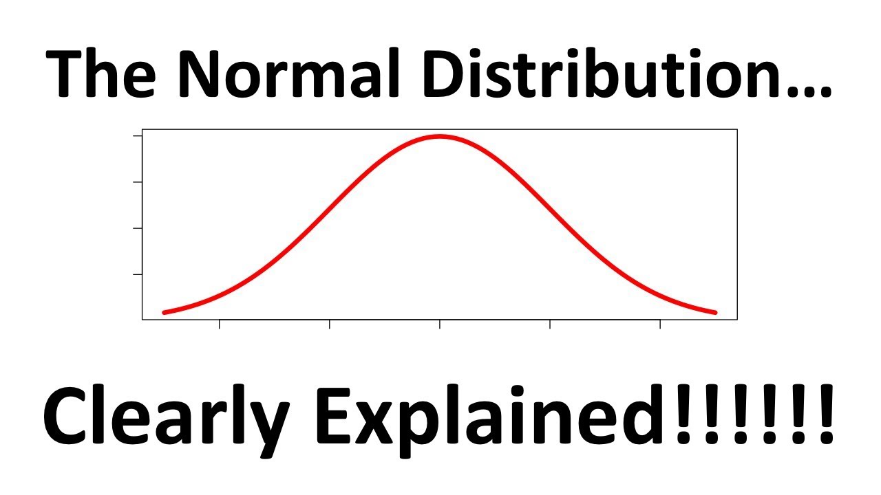
• 📊 Normal distribution, also known as Gaussian distribution, is a probability distribution that is symmetric about the mean.
• 📈 The normal curve is unimodal and bell-shaped, and any specific normal curve is defined by its mean and standard deviation.
• 🔍 The mean, median, and mode of a normal distribution are all equal and located at the center of the normal curve.
• 📚 Changing the mean moves the normal curve along the horizontal axis without altering its shape.
• 📉 Changing the standard deviation affects the 'flatness' or 'stiffness' of the normal curve; a larger standard deviation results in a flatter curve.
• 📉 The empirical rule, or the 68-95-99.7 rule, states that approximately 68% of the data falls within one standard deviation of the mean, 95% within two, and 99.7% within three.
• 📐 For a normal distribution with a mean of 150 and a standard deviation of 3, about 68% of data values fall between 147 cm and 153 cm.
• 📈 Approximately 97.5% of heights are greater than 144 cm when the mean height is 150 cm and the standard deviation is 3.
• 📊 About 2.5% of students have a height greater than 156 cm under the same distribution parameters.
• 🔄 The binomial distribution can resemble a normal distribution when the probability of success is around 0.5 and the number of trials is large.

Q & A

What is the normal distribution?

The normal distribution, also known as the Gaussian distribution, is a probability distribution that is symmetric about the mean. It shows that data near the mean are more frequent than data far from the mean and is represented graphically by a normal curve.

What are the key characteristics of a normal curve?

A normal curve is symmetric about the mean, has a single peak, is unimodal, and is bell-shaped.

How is a normal curve described?

A specific normal curve is described by its mean and standard deviation, which determine its location and flatness.

What happens when you change the mean of a normal curve?

Changing the mean moves the normal curve horizontally along the horizontal axis without changing its shape.

How does the standard deviation affect the normal curve?

The standard deviation affects how flat or steep the normal curve is. A larger standard deviation results in a flatter curve, while a smaller standard deviation results in a steeper curve.

What is the empirical rule or the 68-95-99.7 rule?

The empirical rule states that for a normal distribution, approximately 68% of the data falls within one standard deviation of the mean, about 95% within two standard deviations, and 99.7% within three standard deviations.

What proportion of data falls outside of three standard deviations in a normal distribution?

Only about 0.3% of the data falls outside of three standard deviations in a normal distribution.

In the example given, what proportion of grade n students have a height between 147 cm and 153 cm?

Approximately 68% of grade n students have a height between 147 cm and 153 cm, as these values are one standard deviation away from the mean of 150 cm.

What proportion of students have a height greater than 144 cm according to the empirical rule?

97.5% of the students have a height greater than 144 cm, as 2.5% are below one standard deviation from the mean and 95% are within two standard deviations.

How does the proportion of students with a height greater than 156 cm relate to the empirical rule?

Only about 2.5% of students have a height greater than 156 cm, as this value is three standard deviations away from the mean.

When does a binomial distribution resemble a normal distribution?

A binomial distribution resembles a normal distribution when the probability of success is approximately 0.5 and the number of trials (n) is large.

What factors determine if a binomial distribution can be approximated by a normal distribution?

The binomial distribution can be approximated by a normal distribution if the probability of success (p) is close to 0.5 and the number of trials (n) is large enough.

Outlines

00:00

📊 Understanding the Normal Distribution

This paragraph introduces the concept of the normal distribution, also known as the Gaussian distribution. It's a probability distribution that is symmetric about the mean, indicating that data points close to the mean are more frequent than those far away. The normal distribution is represented graphically by a bell-shaped curve. The shape of the curve is determined by the mean and standard deviation. The paragraph explains that changing the mean shifts the curve horizontally, while changing the standard deviation affects its steepness or flatness. It also mentions the empirical rule, or the 68-95-99.7 rule, which states that nearly all data points in a normal distribution fall within three standard deviations from the mean, with approximately 68% within one standard deviation, 95% within two, and 99.7% within three.

05:00

📏 Applying the Normal Distribution to Height Data

In this paragraph, the script discusses a practical example of the normal distribution by applying it to the heights of grade N students in a school. The distribution is normal with a mean height of 150 cm and a standard deviation of 3 cm. The paragraph calculates the proportion of students with heights between 147 cm and 153 cm, which is one standard deviation from the mean, and estimates this to be approximately 68%. It also addresses the proportion of students taller than 144 cm, which is two standard deviations below the mean, estimating this to be 97.5%. Lastly, it considers the proportion of students taller than 156 cm, which is two standard deviations above the mean, and estimates this to be 95%. The paragraph concludes by noting the resemblance of the binomial distribution to the normal distribution when the probability of success is around 0.5 and the number of trials is large, suggesting the use of normal distribution approximation for such cases.

Keywords

💡Normal Distribution

Normal distribution, also known as Gaussian distribution, is a probability distribution that is symmetric about the mean. It is characterized by a bell-shaped curve, which is the most widely recognized distribution in statistics. In the script, it is described as having data near the mean occurring more frequently than data far from the mean. This concept is central to understanding the video's theme as it lays the foundation for the discussion on how data is distributed in a normal curve.

💡Mean

The mean, often referred to as the average, is the sum of all values in a dataset divided by the number of values. It is a measure of central tendency and is crucial in normal distribution as it represents the center of the distribution. The script mentions that changing the mean moves the normal curve horizontally, illustrating its importance in determining the location of the distribution.

💡Standard Deviation

Standard deviation is a measure of the amount of variation or dispersion in a set of values. A low standard deviation indicates that the values tend to be close to the mean, while a high standard deviation indicates that the values are spread out over a wider range. In the context of the script, it is noted that changing the standard deviation affects the 'flatness' or 'stiffness' of the normal curve, thus influencing its shape.

💡Symmetric

Symmetry in the context of normal distribution means that the left side of the curve is a mirror image of the right side. This property is highlighted in the script as a defining characteristic of normal curves, emphasizing that data points near the mean are more frequent than those further away.

💡Bell-shaped Curve

A bell-shaped curve is a graphical representation of the normal distribution, where the peak of the bell represents the mean, and the tails extend to the left and right. The script uses this term to describe the graphical representation of the normal distribution, which is essential for visualizing how data is distributed.

💡Empirical Rule

The empirical rule, also known as the 68-95-99.7 rule, is a statistical concept that applies to normal distributions. It states that approximately 68% of the data falls within one standard deviation of the mean, 95% within two standard deviations, and 99.7% within three standard deviations. The script uses this rule to provide specific examples of how data is distributed in a normal curve.

💡Mode

The mode is the value that appears most frequently in a data set. In a normal distribution, the mode is the same as the mean, which is also the median. The script mentions this to emphasize the centrality of the mean in normal distributions.

💡Unimodal

Unimodal refers to a distribution having a single peak. The script describes normal distribution as unimodal, meaning it has one peak at the mean, which is a key characteristic that distinguishes it from other types of distributions that may have multiple peaks.

💡Z-Score

A Z-score represents how many standard deviations an element is from the mean. The script discusses the concept in relation to the empirical rule, explaining that data points within certain Z-scores (1, 2, or 3 standard deviations from the mean) represent specific percentages of the data set.

💡Binomial Distribution

Binomial distribution is a discrete probability distribution that models the number of successes in a fixed number of independent Bernoulli trials. The script mentions that when the probability of success is approximately 0.5 and the number of trials is large, the binomial distribution begins to resemble the normal distribution, illustrating the connection between these two types of distributions.

💡Normal Approximation

Normal approximation is a method used to approximate the distribution of a binomial random variable with a normal distribution under certain conditions. The script explains that when the number of trials is large and the probability of success is around 0.5, the binomial distribution can be approximated by a normal distribution, which is useful for simplifying calculations.

Highlights

Normal distribution is symmetric about the mean, showing that data near the mean are more frequent.

Normal curves have the same shape and are symmetric with respect to the middle value.

A normal curve is unimodal and bell-shaped.

A normal curve is completely described by its mean and standard deviation.

Changing the mean moves the normal curve horizontally.

Changing the standard deviation affects the flatness or stiffness of the normal curve.

The mean, median, and mode of a normal curve are all equal and located at the center.

The empirical rule (68-95-99.7 rule) states that almost all data falls within three standard deviations from the mean.

Approximately 68% of data falls within one standard deviation from the mean.

Approximately 95% of data falls within two standard deviations from the mean.

Approximately 99.7% of data falls within three standard deviations from the mean.

The remaining 0.3% of data falls outside three standard deviations from the mean.

The area under the normal curve equals 100%, representing the total proportion of data.

For a normal distribution with mean 150 and standard deviation 3, approximately 68% of students have heights between 147 cm and 153 cm.

For the same distribution, 97.5% of students have heights greater than 144 cm.

For the same distribution, 2.5% of students have heights greater than 156 cm.

Binomial distribution resembles a normal distribution when the probability of success is approximately 0.5 and the number of trials is large.

The closer p is to 0.5 and the larger n is, the more the binomial distribution resembles a normal distribution.

When p is close to zero or one and n is small, the normal approximation would yield inaccurate results.

Transcripts

our lesson for today is about the normal

distribution normal distribution by

definition normal distribution or the

gausian

distribution is a probability

distribution that is symmetric about the

mean showing that data near the mean are

more frequent in occurrence than data

far from the mean it is graphically

represented by a normal

curve so this is an example of a normal

curve so symmetric about the mean so

whatever

manues mean than

those mean note that normal curves have

the same

shape

soer symmetric with respect to the

middle value

it is single Peak

unimodal and it is Bell

shape any specific normal curve is

completely described by giving its mean

and standard

deviation

so or flatness depending on these two

values okay your mean and

your standard deviation so

Al stiffness or flatness so we have here

our normal curve okay mean let's say we

have zero with the standard deviation

equal to

1ue

mean as you can observe changing the

value of mean moves our normal curve

horizontally

how

about

stand deviation

mean normal

curve

flat normal curve as observ example the

mean is located at the center of the

normal curve in fact mean even the

median and the

mode and they are all

equal center of the normal

curve changing the mean without changing

the standard deviation moves the normal

curve along the horizontal

axis okay and changing the standard

deviation affects how flat or stiff the

normal curve is so

lesser value standard

deviation

larger value standard

deviation

flat normal

curve for a normally distributed data we

have this empirical rule or sometimes we

call the three sigma rule or 6895 99.7

rule which states that almost all obser

data will fall within three standard

deviations from the mean so normally

distributed

data

99.7% data within three standard

deviations okay so very small greater

than three standard

deviations

specifically EMP

rule Sigma rule okay

it states

that within one standard deviation from

the mean approximately

68%

dat

okay

orus at within two standard

deviations approximately

95% data

values and three standard deviations

from the mean 99.7% % data

values so remaining

3% more than three standard deviations

from the mean note that proportion is

100% okay

so area normal

curve that is equal to one

100%

proportion

now let's take a look at this example

the distribution of heights of grade n

students in a certain school is normal

with mean equal to 150 and standard

deviation equal to three What proportion

of the grade n students have a height

between 147 cm and 153

CM or What proportion of the students of

a height greater than 144 CM or What

proportion of the student of a height

greater than 156

CM

so proportion my height between 147 and

153 observe that 147 and

153 are one standard deviation from the

mean CU 150 - 3 is 147 150 + 3 is

153 since one St standard deviation sha

from the mean then we say that

approximately

68% of the data values fall within 147

to

153 CM so n Heights no

68% Heights n values 147 to 153 how

about the proportion of students with a

height greater than 144 C CM looking at

our normal curve okay observe that you

one standard deviation

right two standard

deviations meaning from 144 up

to6 95% na Yan okay 95% based on the

empirical rule however P small portion

here okay so 95

that is 5%

okay5 so what is that that is

2.5% 5% so if we have

95 plus

2.5

totalan

97.5%

so

97.5% of the heights are greater than

144

cm and finally What proportion of

students have a height greater than

156 okay so from

here one standard deviation

Yan two standard

deviations so that is

95% so nawan 5% Lang

okay then this

is

2.5% when we deal with a binomial random

variable with large number of

Trials you might observe that

calculating the probabilities will be

too difficult or impossible without the

use of a statistical

tools if we investigate the shape of a

binomial

distribution we can observe that that it

resembles the normal distribution when

the probability of success is

approximately

0.5 and the number of Trials n is large

enough in fact the closer p is to 0.5

and the larger n is the more it

resembles the shape of a normal

distribution

we can observe from these figures how

the values of p and N affects the shape

of the

distribution however how do we determine

if n is already large

enough so depend a probability of

success this is because when p is close

to zero or one and N is small the normal

approximation would yield in accurate

result

figure look at the figure

four okay in

approximate normal

distribution