mod04lec22 - Quantum Generative Adversarial Networks (QGANs)

Summary

The video script delves into quantum machine learning, specifically focusing on quantum generative adversarial networks (GANs) applied to option pricing in finance. It explains the concept of GANs with a generator and discriminator, aiming to produce data indistinguishable from real samples. The script discusses a quantum approach to address data loading challenges, using a quantum generator and classical discriminator. It showcases how this framework is applied to European call option pricing, demonstrating faster convergence compared to classical Monte Carlo simulations. The script also includes a demo of quantum GANs for finance and a simulation of molecules using the Variational Quantum Eigensolver (VQE), emphasizing the practical application and potential of quantum computing in various fields.

Takeaways

• 🧠 The script discusses the application of Quantum Generative Adversarial Networks (GANs) in finance, specifically for option pricing.
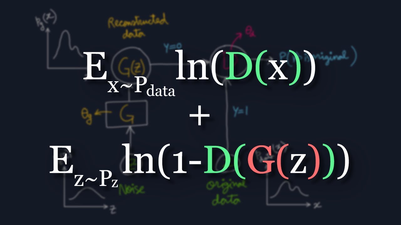
• 🤖 It explains the concept of GANs, which involve two neural networks: a generator that creates data samples and a discriminator that tries to distinguish between real and generated samples.
• 📈 The goal of the generator is to produce samples that are indistinguishable from real data, thus 'fooling' the discriminator.
• 💡 The script highlights a paper that addresses the 'data loading problem' in quantum computing, aiming to mimic data distributions without needing to load the exact classical data into quantum states.
• 🌐 It introduces a quantum framework where the generator is quantum (using variational quantum circuits) and the discriminator remains classical.
• 💼 The application demonstrated is European call option pricing, where the quantum approach is used to simulate the distribution of spot prices and calculate expected payoffs.
• 📊 The script shows a comparison between quantum computing and Monte Carlo simulations, with quantum showing faster convergence and lower estimation errors.
• 🔬 The demo includes a practical example of using the quantum GAN framework to price options, with the potential for significant efficiency gains over classical methods.
• 🔄 The script also touches on the broader context of quantum computing, including the NISQ (Noisy Intermediate-Scale Quantum) era and the importance of variational quantum algorithms.
• 🚀 Lastly, it emphasizes the rapid evolution of quantum hardware and the active research in areas like cost function optimization, Hamiltonian mapping, and quantum-aware classical optimizers.

Q & A

What is the main concept behind Generative Adversarial Networks (GANs)?

The main concept behind GANs is to have two neural networks, a generator and a discriminator, competing against each other. The generator creates data samples, while the discriminator tries to distinguish between these generated samples and real data samples. The generator's goal is to produce samples that are indistinguishable from real data, effectively 'fooling' the discriminator.

How does the quantum version of a GAN differ from the classical one?

In the quantum version of a GAN, the generator is a quantum circuit that produces quantum states approximating the distribution of the training data, while the discriminator remains a classical neural network. The quantum generator uses parameterized quantum circuits to generate states that encode the probability distribution of the data.

What is the significance of the data loading problem in quantum computing?

The data loading problem refers to the challenge of efficiently translating classical data into quantum states. It's significant because even if quantum algorithms can provide exponential speedups, if loading classical data into quantum states requires an exponential number of gates, it negates the potential speedup. The paper discussed in the script addresses this problem by aiming to mimic the data distribution rather than loading the exact data.

How does the quantum GAN framework handle the data loading problem?

The quantum GAN framework handles the data loading problem by focusing on mimicking the distribution of the data rather than loading the exact classical data into quantum states. This approach allows for a more efficient translation of data into a quantum context, sidestepping the need for complex gate operations.

What is the role of the variational quantum circuit in the quantum GAN?

The variational quantum circuit in the quantum GAN serves as the quantum generator. It is a parameterized quantum circuit that is trained to generate quantum states whose probability distributions closely resemble the training data. This circuit is essential for encoding the data distribution into quantum amplitudes.

How is the payoff in a European call option calculated?

The payoff in a European call option is calculated as the maximum of the difference between the spot price at maturity (S_t) and the strike price (K), or zero. If the spot price at maturity is higher than the strike price, the payoff is positive; otherwise, it is zero.

What is the advantage of using a quantum approach over classical Monte Carlo simulations for option pricing?

The quantum approach has a convergence rate that scales polynomially faster than the Monte Carlo method, which scales with 1/√n. This means that the quantum approach can achieve the same level of accuracy with significantly fewer samples, offering a potential quantum advantage in computational efficiency.

What is the key takeaway from the paper on quantum GANs for finance?

The key takeaway is that the quantum GAN framework can effectively mimic the distribution of financial data, allowing for more efficient computation of expected payoffs in option pricing. This approach demonstrates a potential quantum advantage over classical methods, particularly in the context of complex financial simulations.

How does the quantum GAN framework encode the spot price information?

The quantum GAN framework encodes the spot price information into the quantum state's basis states, where each basis state represents a number in the domain of the data. The probability distribution of the spot price is then embedded into the amplitudes of these states, allowing for the generation of a distribution that can be used for financial calculations.

What are some of the active research areas in variational quantum algorithms?

Active research areas in variational quantum algorithms include defining cost functions, mapping Hamiltonians, exploring useful ansatze, utilizing gradients, and developing quantum-aware classical optimizers. These areas are crucial for improving the efficiency and applicability of variational quantum algorithms.

Outlines

00:00

🧠 Introduction to Quantum Generative Adversarial Networks in Finance

The paragraph introduces the application of quantum generative adversarial networks (GANs) in the context of finance, specifically for option pricing. It explains the concept of GANs where a generator network creates data samples, and a discriminator network tries to distinguish between real and fake samples. The goal is for the generator to produce samples so realistic that the discriminator cannot differentiate them from actual data. This framework is then applied to finance, aiming to mimic data distributions without needing to load the exact classical data into quantum states, addressing the data loading problem that plagues quantum algorithms. The paper referenced discusses a quantum generator and a classical discriminator, using variational quantum circuits to generate data distributions that are then used in financial modeling.

05:00

🔄 Quantum Circuit Design for Generative Models

This section delves into the specifics of the quantum circuit used in the generative model. It describes a parameterized quantum circuit with rotations and entangling gates, which is repeated multiple times to refine the output. The circuit's output, represented by a trial state, is then measured to obtain a probability distribution. This distribution is encoded in the amplitudes of quantum states, allowing for the generation of data samples that mimic a given distribution. The paragraph also discusses how this quantum-generated distribution is applied to European call option pricing, where the spot price is encoded into the quantum state, and the expected payoff is calculated using amplitude estimation techniques. The results show that the quantum approach can converge faster than classical Monte Carlo simulations, offering a potential quantum advantage.

10:01

📈 Demonstrating Quantum Advantage in Option Pricing

The paragraph showcases a demonstration of using the quantum generative model for option pricing. It presents a graph that compares the payoff and probability distribution of the spot price between quantum and Monte Carlo simulations. The quantum simulation is shown to converge much faster to the expected value with fewer samples, highlighting the potential efficiency of quantum computing in financial applications. The paragraph emphasizes the practical implications of this faster convergence, suggesting that quantum computing could significantly reduce the computational resources needed for financial modeling and decision-making.

15:02

🌐 Simulating Molecules Using Variational Quantum Eigensolver (VQE)

This section shifts focus to another application of quantum computing: simulating molecules using the Variational Quantum Eigensolver (VQE) algorithm. It provides a brief overview of the process, including initializing the quantum circuit, encoding the molecular information, and running the VQE algorithm to calculate the energy of the molecule at different distances. The paragraph also touches on the challenges and considerations in running VQE, such as choosing the type of entanglement and dealing with noise in quantum hardware. The narrative encourages hands-on experimentation with VQE through provided links to Jupyter notebooks, allowing users to run simulations and explore the practical aspects of quantum chemistry.

20:04

🔬 The Evolution and Challenges of Variational Quantum Algorithms

The final paragraph summarizes the current state and future prospects of variational quantum algorithms (VQAs). It acknowledges the rapid evolution of quantum hardware and the ongoing research into VQAs, which are crucial for handling noise and errors in the current noisy intermediate-scale quantum (NISQ) era. The paragraph outlines active research areas such as cost function design, Hamiltonian mapping, and quantum-aware classical optimizers. It also discusses the challenges faced by VQAs, including trainability, measurement efficiency, and accuracy. The speaker expresses optimism about the potential of VQAs to revolutionize various fields and encourages further exploration and career development in quantum computing.

Keywords

💡Quantum Generative Adversarial Networks (QGANs)

Quantum Generative Adversarial Networks (QGANs) are a type of quantum machine learning model inspired by classical GANs. In the video, QGANs are used to mimic complex data distributions, which is crucial for applications like option pricing in finance. The script discusses how QGANs consist of a quantum generator and a classical discriminator, where the generator's role is to produce data samples that are indistinguishable from real data, as per the adversarial training process.

💡Generator

In the context of GANs, the 'generator' is a neural network that creates new data samples. In the video, the generator is adapted to a quantum framework, suggesting a quantum version that can generate data samples with distributions close to real-world data. This is showcased in the application of QGANs to finance, where the quantum generator learns to mimic financial data distributions.

💡Discriminator

The 'discriminator' is another neural network in GANs that evaluates data samples, distinguishing between those generated by the generator and real data. In the video, the discriminator remains a classical neural network, tasked with identifying whether data samples are real or fake, thus providing feedback to the quantum generator.

💡Data Loading Problem

The 'data loading problem' refers to the challenge of efficiently translating classical data into a quantum state. The script highlights this as a significant issue in quantum computing, especially when trying to leverage quantum speedups. The paper discussed in the video addresses this problem by focusing on mimicking data distributions rather than exact data loading.

💡Variational Quantum Algorithms (VQAs)

Variational Quantum Algorithms are a class of quantum algorithms that use parameterized quantum circuits to find solutions to problems. In the video, VQAs are central to the quantum generator's operation in QGANs, where they are used to create a quantum state that encodes the data distribution. VQAs are highlighted as a practical approach in the current noisy intermediate-scale quantum (NISQ) era.

💡European Call Option

A 'European Call Option' is a type of financial derivative that gives the holder the right, but not the obligation, to buy an asset at a specified price (the strike price) on or before a certain date. In the video, the application of QGANs to finance involves pricing this type of option, where the quantum approach is used to model the underlying asset's price distribution and calculate the option's expected payoff.

💡Amplitude Encoding

In quantum computing, 'amplitude encoding' is a method of representing classical data in quantum states through the amplitudes of quantum bits (qubits). The video describes how amplitude encoding is used in the quantum generator to embed the probability distribution of financial data into the quantum state, which is then measured to sample from the learned distribution.

💡Quantum Advantage

The term 'quantum advantage' refers to the ability of quantum computers to solve certain problems more efficiently than classical computers. The video script discusses the potential quantum advantage in the context of option pricing, where the quantum approach is shown to converge faster than classical Monte Carlo simulations, indicating a polynomial speedup.

💡Convergence Rate

The 'convergence rate' in the context of algorithms is the speed at which a solution or output approaches the true or desired value. The video emphasizes the superior convergence rate of the quantum approach compared to classical Monte Carlo methods, showcasing how quantum algorithms can achieve more accurate results with fewer samples or iterations.

💡Quantum Hardware

The script mentions 'quantum hardware' as the physical devices that implement quantum computing, such as quantum processors. The video demonstrates how these devices can be used to run quantum algorithms, like those for option pricing, potentially offering advantages over classical computing hardware due to their ability to perform certain calculations more efficiently.

💡Noisy Intermediate-Scale Quantum (NISQ) Era

The 'NISQ era' refers to the current phase of quantum computing development, characterized by devices that are noisy and have a limited number of qubits. The video discusses how variational quantum algorithms are particularly suited for this era, as they can operate with the shallow circuits necessary to mitigate the effects of noise in current quantum hardware.

Highlights

Overview of quantum generative adversarial networks applied to option pricing and finance.

Introduction to generative adversarial networks (GANs) with two neural networks: generator and discriminator.

The generator's goal to produce samples indistinguishable from real data.

The discriminator's role to identify real from fake data samples.

Loss functions for the generator and discriminator in the GAN framework.

Quantum approach to address the data loading problem in quantum computing.

Quantum GAN framework with a quantum generator and a classical discriminator.

Variational quantum circuit design for the quantum generator.

Encoding the probability distribution into the quantum state amplitudes.

Application of the quantum GAN framework to European call option pricing.

Demonstration of faster convergence in quantum simulations compared to Monte Carlo methods.

Quantum advantage in finance through polynomially faster convergence rates.

Practical demonstration of quantum GANs for finance with IBM Quantum Lab.

Variational Quantum Eigensolver (VQE) for simulating molecules.

Programming quantum circuits in Python for VQE.

Challenges and active research areas in variational quantum algorithms.

Potential use cases of variational quantum algorithms across various industries.

The current state of practical quantum computing and its future trajectory.

Transcripts

[Music]

now that we have seen the variation of

quantum migrant solver in detail we

cannot do a quick overview of quantum

generate generative adverse serial

networks as applied to option pricing

and finance this will be a very high

level cursor review uh the idea being

that we want to give a flavor of how

this gets applied in an application

context in finance

so as a background um the idea of

generative advice serial networks is uh

is to have two neural networks naturally

this comes from the machine learning

space you have two neural two neural

networks called the generator and the

discriminator

generator generates the data samples the

discriminator

takes the data samples generated by the

generator along with the training or

real data samples and it's supposed to

be able to distinguish between the data

samples that it got

mark it real or fake

what generator wants to do is ultimately

generate the samples such that the

distribution is as close to the real

data samples and so the discriminator is

not able to tell whether it is a real

data or a fake data

and so this goes about

in you know in a it's much like a two

player game in game theory and uh

eventually the generator learns the

distribution and is able to

make the training data as close as

possible

so the loss functions defined here um

our

the expectation value of the prior uh

where

z or z

is from the prior distribution this is

the generator's loss function uh this is

in the non-saturating loss kind of

framework

where theta

is for the generator distribution

and then the results the data samples

generated then goes into the

discriminator and what

what this wants to do is

maximize the chance of the discriminator

tagging it as real which means that it's

able to fool the discriminator saying

that the data samples are actually real

in a sense the discriminator is not able

to tell

the two distributions apart and you want

to maximize that

from a generator standpoint and

discriminator standpoint is the other

one so we want to be able to identify

the fake ones as fake and the real ones

as real so now you have a conflicting

thing so you have a push and pull coming

in and which is what mimics the

two-player

game from game theory and it is

equivalent to the national equilibrium

where the two of these players are

trying to maximize

their objectives and eventually the

result

will be such that the generator is able

to generate samples so that it's as

close to the training data as possible

so the paper that we are referring to is

uh

we have the snapshot on the top left in

the orange box that's the actual paper

um so the idea the key takeaways

is the context is very important to

understand to this paper this is our the

context is slightly different from the

application itself

there are many algorithms that have come

before that

involve what is called as a data loading

problem

some of the algorithms like hl

have exponential speed up compared to

the classical counterpart but there is a

big hole in that argument that being

that data loading so when you have the

classical data

can you load that into a quantum state

efficiently or not what was shown later

was that that loading particular problem

uh takes exponentially many number of

gates to translate the classical data

into quantum and thus um

eventually

negating the exponential speed up that

potentially some of these algorithms

like etcetera

so this data loading problem is an open

problem and this particular paper

addresses that particular problem at

hand um so what it's trying to do with

the quantum grants framework is uh the

data set that we have at hand can i

mimic it at least in the distribution

sense as close as possible rather than

having to actually load the real data

in in exact form so at least can i mimic

the distribution as close as pos

possible and the framework that they

adopted in this paper was

the same generated discriminatory type

framework um

here the generator is

quantum

that discriminator remains classical

neural network so the classical neural

network discriminator remains but the

generator is replaced by a quantum

framework so you can see at the bottom

left um a quantum generator uh you can

see that it's a very

by now um a very common variational

quantum algorithm that you would have

seen you have these

rotation the parameter parameterized

quantum circuit with rotations and they

use the ry rotation and then you have

the entangling gate followed by the r

way rotation and there are n number of

times that you do it so um you have the

initial rotation followed by the

sandwich of these entangling followed by

single qubit gates

k times and that's what this one is this

is what we had seen in the previous

sections as well

and you get the

g of theta which is the trial state at

the end and in order for you to get the

result so you just do the measurement so

the way it is encoded is each basis

state so um if you look at the

indices here it goes from 0 to 2 power n

minus 1. so this particular state

encodes

the natural domain value that it encodes

goes is assumed to go from 0 to 2 power

n

minus 1 it directly encodes that p theta

of j is essentially telling you for that

particular basis where each of them

represents

each basis state represents a number for

example

in the sampling x um

sample data from 0 to 2 power n minus 1

each basis states corresponds to a

particular number there and p of theta

of j represents the probability of the

distribution of that particular value in

it so that's how it gets um the

distribution part gets embedded into the

amplitude of that particular state and

therefore the state gets encoded here

and then use when you do measurement you

get the right probability distribution

for the values

that you had at hand

so what they did then is that once you

have this generator framework and

eventually it gets trained and you you

generate the distribution uh you know

finally after training you get the g of

theta the distribution what they did was

they applied this in the european call

option

spot pricing contacts what it is is less

important i have a link here that you

can go read up on what this call option

is all about but the idea there is there

is a

in the financial market sense

there is uh

you you

price k is what you

buy the spot option you are not

necessarily um

and the value of that option can go up

in time the maturity time is t

so the value of it at the maturity st

the difference of it means

the

the payoff

if it is

more the sft is more than what you are

buying for then you get a payoff which

is positive and if it is negative you

you are guaranteed that you don't

necessarily have to buy that one so it

is

zero here so

what this payoff is is essentially

maximize um the spot price at maturity

which is s of t to the current price

that you are quoting and the difference

of it and you want to maximize that

that's what this particular option

pricing is about

what they did was to encode

the spot rising

part of it in g of theta remember i

mentioned that the actual data the

domain of it goes from 0 to 2 power n

minus 1 that goes directly encoded into

the state the basis state

and note that the

n qubits means that the basis state has

2 power n combinations so you can sort

of each state represent a particular

number so you can sort of encode it into

it

and they had a prior work which

basically can do based on amplitude

estimation approaches um go from

the spot price value and they and then

you get the results which is essentially

the expected payoff uh which is what you

get at the end so what they did is they

use the data loading problem what they

solved here

they applied the data loading in this

case they loaded the spot price

information into the earlier work that

they had done where

they had shown how to do the computation

of expected payoff

this is the circuit that is based on the

amplitude estimation approach

so they encoded they get the payoff and

then they showed that you could then

simulate the results to see

what is the value of payoff

the key important value proposition is

that the earlier work that they did

here uh all these analysis uh invariably

involves when the distribution is

becomes fairly complex the only way to

do that in the classical sense is to do

a multicordless simulation

we know from

our prior knowledge the monte carlo

simulation the convergence goes like 1

over square root of n

in this work um

the prior work that i shown here they

showed that

using this quantum approach the

convergence goes more like 1 over n

which means that the convergence is

polynomially faster

than the monte carlo approach

which is the key value proposition of

all of this so

so now you have an end to end thing

where you can load the data from the

classical data into the quantum at least

in the distribution sense and then

perform your expectation value

calculation in the quantum sense and

generate the result and we know from the

prior work that this computation is

polynomially faster than um the monte

carlo which means that the convergence

is much sooner and you're likely to get

to the results with less number of

sampling than you would have to do with

the monte carlo approach uh we will see

uh

couple of demonstrations uh this

demonstration for this uh shortly uh

very intuitive one uh the picture here

is showing on the uh

the second um y-axis is the payoff which

is the blue line and this is the

probability distribution for the spot

price which is the x axis here

the in this particular example the

initial spot price was fixed at 2

and then you have the expected gain and

as you can see it grows up so in the

simulation uh i will show you uh

this particular simulation and also it

shows uh the convergence how quickly it

converges uh to the value of interest

and thus demonstrating the value

proposition

or a potential quantum advantage that

you can get

using the quantum hardware to solve this

particular problem

now we're going to go into the demo part

of it

i'm going to cover a couple of them um

so i'm going to first talk about

the

the quantum gangs since we just covered

it um i will show the demo of this you

can find this in this link and then i

will show you the vqa

code uh just to indicate um that it is

highly programmable and it's easy to go

play with so i encourage you all to go

take a look at that

so i've opened the link that i had in

that chart here this indicates uh this

is uh

for the work for the quantum grants work

that i just talked about so we're going

to cover that first the finance one

um so the example um

we talked about in this in this case is

you can choose the spot price and what

you are doing is in the future when the

price increases you're gonna get profit

but if the price reduces you're not

gonna you have the option of not selling

it for that particular price which means

that you don't lose it and that's the

idea of this call european call option

so here for example um the spot price is

set at 1.9

dollar 1.9

so let's run the

test circuit

so

this one is the payoff payoff is the

expected

gain of doing that

the important part is

the white line is the

quantum and the gray line is monte carlo

and

since these numbers these simulations

are for very small set of values we can

do an exact calculation too which is the

pink reference line

so here you can see the

quantum

calculation converges pretty quickly the

monte carlo goes up and down a little

bit and then converges

on the right is the estimation error

which is more relevant on the x axis in

this particular plot is the number of

samples

what you can see is the white line is

the quantum and the gray line is the

monte carlo simulation

so you can see that the the estimation

error from quantum drops quite rapidly

compared to the monte carlo i told you

that the earlier result had demonstrated

the convergence rate of mono rain for

quantum as against one over square root

of n for monte carlo so that is evident

in this particular example here so for

example if your error threshold i don't

know if you can see this number

were

0.009

i think that's what this one is

let's say you had that as the threshold

you would get that hit the threshold in

this particular example with the

sampling of 256

and you would get to that

error threshold only in the classical

monte carlo case only when you sample

2048

samples so this shows a big difference

this could be

really important in the context of

finance sector so

so based on the threshold and the

convergence is much faster compared to

the

classical monte carlo approach

you can go play with different values

of

the spot price and give it a run and you

will see a consistent behavior in terms

of the convergence

in this example you can see that the

quantum converges soon

the variance in the classical is much

broader here

and you can see that it achieves the

lower threshold

we run it for 2048 samples in both but

you can see if we had a threshold

value for example in this horizontal you

get it in 256 but to get to that in

monte carlo actual monte carlo you have

to sample 2048

samples

the structure of the algorithm there is

a broader

structure you have the payoff circuit

that i was telling you about from before

remember the amplitude distribution

based approach and then you have the

distribution

technique which is what we talked about

in quantum gas to get the data in the

data loading problem portion which is

what this one is and then you have the

payoff calculation portion which is the

second part

now i'm going to go into

the simulation simulating

molecules using vqe we talked about this

in quite detail

in our presentation i will just go over

this particular

thing you can open this as a jupiter

notebook and actually run them so all

you have to do is click it and it opens

in ibm quantum lab if you haven't uh if

you create an id with

quantum computing

ibm.com um it's as simple as logging

into it and then

you you can go run them i'm not going to

do that now but i just will show you

walk you through this particular

textbook page we have covered all this

in quite detail so i'm not going to talk

about these technical part of it as much

but i want to show the programming part

of it a little bit

um so here is where the quantum circuit

gets initialized these are all one time

thing these are all abstracted as you

can see in the

in a function

so this is the variational form that we

talked about you can program it is the

quantum and this is the classical

register this is the quantum circuit

that you are defining and these are the

parameters these are the u3 parameters

and you measure them

remember um

the big level picture is you have the

classical optimizer and that's what this

one is here they are using cobala as the

optimizer um

you get the variational form this is the

quantum circuit that you want to run you

then compile it and assemble it and you

set up

the background on the back end that you

want to run it in

and then you get the distribution

okay

so note that

you had the variation part and then the

entangling variation and dangling and so

forth the parameter is part and then the

entangling part the parameter is part

and tangling part so there are two

different kinds of entangling that you

can do a linear or a full and this is

something that you can play with

so linear means that uh as you can see

you have in this example they are

showing c naught so you have the c

naught um with in this example they are

showing four qubits uh so you have c

naught uh one two zero two one one two

two two two three full means all

combinations of us not so

one two two one two three one two four

two two three two two four two two so

this is what the full ways uh naturally

the linear uh has lesser number of c

naught which means it's less erroneous

however the full entanglement

will take you to much more complex

entanglement and as you can see with

when you do these

mini c naught in frontal entanglement it

gets much more deeper the number of

layers of quantum circuit increases

we want to keep it shallow as well so

there is a trade-off

between these things

if your hardware is

more

has a more longer lifetime you can

potentially look at full entanglement if

you have a shorter lifetime you would

want to make do with linear entanglement

these are the parameters that you need

to tweak and play with

then

this is where you

encode your circuit so this one is

showing the lithium hydride molecule

from the paper

so what this one is showing is this is

the lithium atom

and then this is the hydrogen atom

lithium is in origin 0 0 0 think of this

is x y and z axis and hydrogen is the

one that is moving so it's fixed in the

x and y plane

but moves only in one direction which is

the z plane and that's the

difference remember the in vqa we showed

the um energy profile so if you have

atoms closer you have higher energy and

then at some point it starts dropping

and when it moves away farther out then

the energy also flattens out

so what they do is they play it in they

change the distance in one direction the

z direction

all these are details here which i'm not

going to talk about

but basically here is the fermionic

operator

that we talked about remember

we have to go from the fermionic

hamiltonian to the qubit hamiltonian so

here is where you get the fermionic

operator

and then

you will have to go do the mapping

so here is where the mapping happens

remember

there are many mappings available there

is jordan wigner mapping bravikit and

here they are using parity this is where

the fermionic operator becomes a cubit

hamiltonian and that's what this one is

so that's how the encoding happens

and then um

you have the this is the main loop this

is the loop where you have the classical

quantum back and forth happening um so

you have the sl sls qp optimizer so

cobella was used for the exact solution

um that for the reference and this is

the actual optimizer used

for the vqe

for different distances remember the

x-axis is the distance we are trying to

compute the

energy

you run it for each of the distances

you calculate the value

uccd is the onsites which is coming from

quantum chemistry it's a very famous

answer from quantum chemistry uh so we

are leveraging that particular answers

um for our calculations and then we just

call vqe um send the qubit hamiltonian

the variational form which is the uccd

and the optimizer the classical

optimizer so this is the main loop that

we are talking about here

and then you calculate the results and

for different distances what is the

energy and what is the exact energy

remember the cobala was used to

calculate the exact energy because this

is a very small molecule which is

simulatable efficiently in classical

this is just for reference and when you

generate that

we get the plot very similar to what we

had

shown in in our presentation this is the

exact energy and the vq energy much

quite exactly so it's indistinguishable

in this particular plot

so you have

so this is

i think i believe this one did not have

the noise i believe they run it with

noise as the next step so you can play

with the

different simulator you can also run it

when actual hardware so here they are

running it in simulator you can choose

to run it in actual hardware and see the

results

so it will be interesting for you to see

how exact the results get

here as i mentioned in the particular

presentation they are using spsa

and this is the number of iterations you

can play with all of them the type of

entanglement that you want to use

here is the vqe as i was telling you

about and you can run it and generate

the results

so it's fairly intuitive it's

programmable in python

and it's fairly high level very

there is a portion where you need some

knowledge but there is also a main loop

which is fairly independent of any uh

significant knowledge of quantum

that you need to do in order to run this

so now that we are done with both these

demos i want to finally summarize

um

we are an interesting uh

point in the journey

uh programming a quantum computer now is

a reality um

and it's fairly advanced already

um and then we are in a generation that

is beyond just experiments now we are in

what is called as the broadly called as

a niskira this will be there for some

time to come uh till such time the

errors are fairly small we are still

orders of magnitude of a

and till such time that the fault

tolerant

quantum computing takes shape we are

going to be in this era and also the

knowledge that we are going to gain

along the way is likely to continue

beyond the niskera 2.

what also needs to be mentioned is

hardware is evolving quite rapidly

exponentially fast we saw that early

the lifetime is increasing quite bad the

noise profiles are reducing quite a bit

all the trend lines are good but still

it's in the regime that will be called

as noisy it's not still at a fault

tolerant threshold we are still as i

mentioned orders of magnitude away

so how do we do computation efficiently

in this particular context is what is

the challenge

traditional algorithms will not be

practical

because it doesn't deal with noise and

the way it does the computation assumes

that the qubits are clean that's not so

in reality at this point in time so they

don't map well so variational quantum

algorithms are the mainstay in this

particular era and possibly beyond as

well and all the efficiencies that we're

going to develop is going to likely to

carry over too

and all the new knowledge is that we're

learning

the variational quantum algorithms are

a hybrid algorithm it's a classical

quantum algorithm

with

shallow depth circuit it's an important

piece the shallow depth part

given that it's noisy we can't afford to

be very deep quantum circuit

there are a lot of areas of active

research in this area including cost

function how do you define the cost

function um there is an active research

there how do you map the hamiltonian

that's another active area of research

what kind of handsets will be useful

how to use the gradients what kind of

classical optimizers are quantum aware

are sensitive to the quantum

requirements that's another active area

of research there is lot of

things that are being looked at and

conjectured and also proven

and there are many many challenges also

along the way as i described there is a

trainability part

how do you what are the

potential barriers to entry the parent

plateau being one significant portion of

them efficiency how well can you do the

measurement um and then the accuracy

part

all these are challenges that

variational quantum algorithms needs to

come about

what has happened in the last few years

is there are many flavors of these

algorithms that have come about based on

the particular requirement of a problem

and many more are being explored

as we speak

potential use cases has exploded in the

last few years

spanned areas of finance natural

sciences l senses manufacturing and this

by no means exhaustive there are many

many more explorations being happen to

look at the problem context how quantum

affects a particular vertical a

particular problem

naturally you would want to go look at

problems that are hard to solve

classically and see if you can solve it

in quantum mechanical in the quantum

computing context and within the quantum

computing context is there a variational

form because variational form is what is

more practical at this time and so

figuring out that kind of a dynamic

is what is currently

the state of the art and there are many

more explorations happening at this

uh i hope uh this particular

introduction to this variation

algorithms gave a flavor for what is

happening in uh in quantum computing the

practical side of quantum computing at

this time i hope many of you find this

useful and i hope many of you take this

journey in

in exploring this space and hopefully

make a career in this area as well i

wish you all the very best and hope

we get to have more such conversations

in the future thank you