Vibration Analysis for beginners 5 (Rules for evaluating machine vibration, Signal path from sensor)
Summary
TLDR本视频是《振动分析入门》系列的第五部分,主要介绍了模拟信号通过模数转换器(A/D)转换为数字信号的过程。强调了采样和量化的重要性,并解释了混叠现象及其预防方法。通过傅里叶变换(FFT)将信号转换到频域,分析振动信号的频率成分。视频还介绍了机器故障和轴承分析的基础知识,包括不平衡、不对中、松动等故障的检测方法以及共振和轴承故障频率的识别。
Takeaways
- ⏲️ 振动传感器的模拟信号需要通过模数转换器(A/D转换器)转换为数字信号才能进行分析。
- 🔄 数字化信号是对输入信号的描述,但并不完全等同于原始信号,重建的模拟信号与原始信号相似但存在差异。
- 📈 采样是将信号的时间轴分成均匀的段,并从每个段中取样,以防止混叠现象。
- 🔍 为了防止混叠,使用低通滤波器确保高于采样频率一半的频率不会进入转换器。
- 🎞️ 混叠现象的一个常见例子是快速旋转物体的电影拍摄,如飞机螺旋桨看起来旋转速度异常慢或反向旋转。
- 📊 通过给定的最大频率(fmax)和测量样本数,可以计算测量持续时间。
- 🔢 量化是将采样值在垂直轴上调整以适应处理数字信号的设备有限的精度。
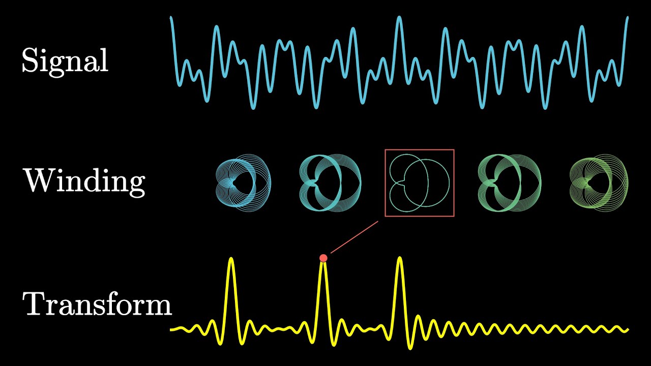
- 📊 频谱分析揭示了组成振动信号的频率,通过快速傅里叶变换(FFT)计算。
- 🛠️ 振动分析可分为机械故障分析和轴承分析,包括不平衡、不对中和机械松动等基本机械故障。
- 🔧 轴承故障发生在高频范围,通过信号解调来识别特定的轴承故障频率。
Q & A
为什么振动传感器的信号需要通过模数转换器转换成数字形式?
-振动传感器的信号是模拟形式的,为了在分析器中使用,必须转换成数字形式,因为数字信号可以被计算机和其他设备处理。
模数转换过程中的采样是什么?
-采样是将信号的时间轴分割成均匀的小段,并从每一段中取样,这样可以得到一组离散的点,这些点的间隔对应于采样频率。
什么是混叠现象,它如何影响信号的转换?
-混叠现象是指当原始连续信号包含高于采样频率一半的频率时,信号在转换过程中会被扭曲。为了防止混叠,使用低通滤波器确保高于采样频率一半的频率不会进入转换器。
为什么在进行振动测量时,采样频率要高于最高捕获频率的2.56倍?
-这是基于快速傅里叶变换(FFT)的工作原理,采样频率是最高捕获频率的2倍可以提供抗混叠保护,而2.56倍则是一个标准,可以更有效地防止混叠。
量化在数字信号处理中起什么作用?
-量化是因为计算机和其他处理数字信号的设备只能以有限的精度表达数字,所以必须在垂直轴上调整采样值,将采样值分配到特定的容差带内。
什么是时间域和频率域,它们在振动分析中有什么作用?
-时间域是信号的时波形表示,而频率域是通过FFT计算得到的信号的频谱。频谱可以揭示组成振动信号的频率,提供比时间域更丰富的信息。
什么是泄漏现象,它是如何影响FFT计算的?
-泄漏现象是指当信号非周期性时,能量会“逃逸”或“泄漏”到几个接近实际频率的谱线上,导致谱线在多个线上扩散。为了减轻泄漏,可以使用窗函数使信号人为地变得周期性。
机器机械故障分析和轴承分析在振动分析中有什么区别?
-机器机械故障分析主要关注低频范围内的不平衡、不对中和机械松动等问题,而轴承分析则关注高频范围内的轴承故障,这些故障通常由球的冲击引起。
如何通过振动测量来检测机器的不平衡故障?
-如果频谱中显示速度频率处有单一的高线,这通常表示不平衡故障。例如,如果频谱中只有25Hz处有一条高线,计算25Hz乘以60得到1500RPM,如果机器的实际速度确实是1500RPM,则故障为不平衡。
轴承故障频率是如何确定的,它与轴承的振动频率有什么关系?
-轴承故障频率是由轴承的球冲击引起的振动冲击(轴承音调)的重复频率确定的。轴承故障频率不会出现在轴承的频谱中,只有球冲击产生的振动频率(轴承音调)是可见的。
信号解调在轴承故障分析中起什么作用?
-信号解调用于识别故障频率。它包括去除低于500Hz的频率(高通滤波器),并使用包络检测人为地向信号添加能量,然后使用FFT处理信号以创建频谱。
Outlines

هذا القسم متوفر فقط للمشتركين. يرجى الترقية للوصول إلى هذه الميزة.
قم بالترقية الآنMindmap

هذا القسم متوفر فقط للمشتركين. يرجى الترقية للوصول إلى هذه الميزة.
قم بالترقية الآنKeywords

هذا القسم متوفر فقط للمشتركين. يرجى الترقية للوصول إلى هذه الميزة.
قم بالترقية الآنHighlights

هذا القسم متوفر فقط للمشتركين. يرجى الترقية للوصول إلى هذه الميزة.
قم بالترقية الآنTranscripts

هذا القسم متوفر فقط للمشتركين. يرجى الترقية للوصول إلى هذه الميزة.
قم بالترقية الآنتصفح المزيد من مقاطع الفيديو ذات الصلة

Vibration Analysis Focusing on the Spectrum (Remastered)
But what is the Fourier Transform? A visual introduction.
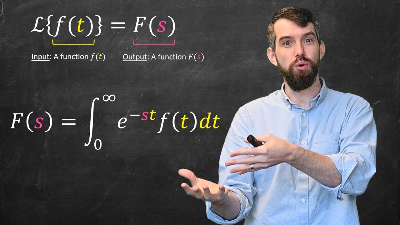
Intro to the Laplace Transform & Three Examples

What is Hashing? Hash Functions Explained Simply
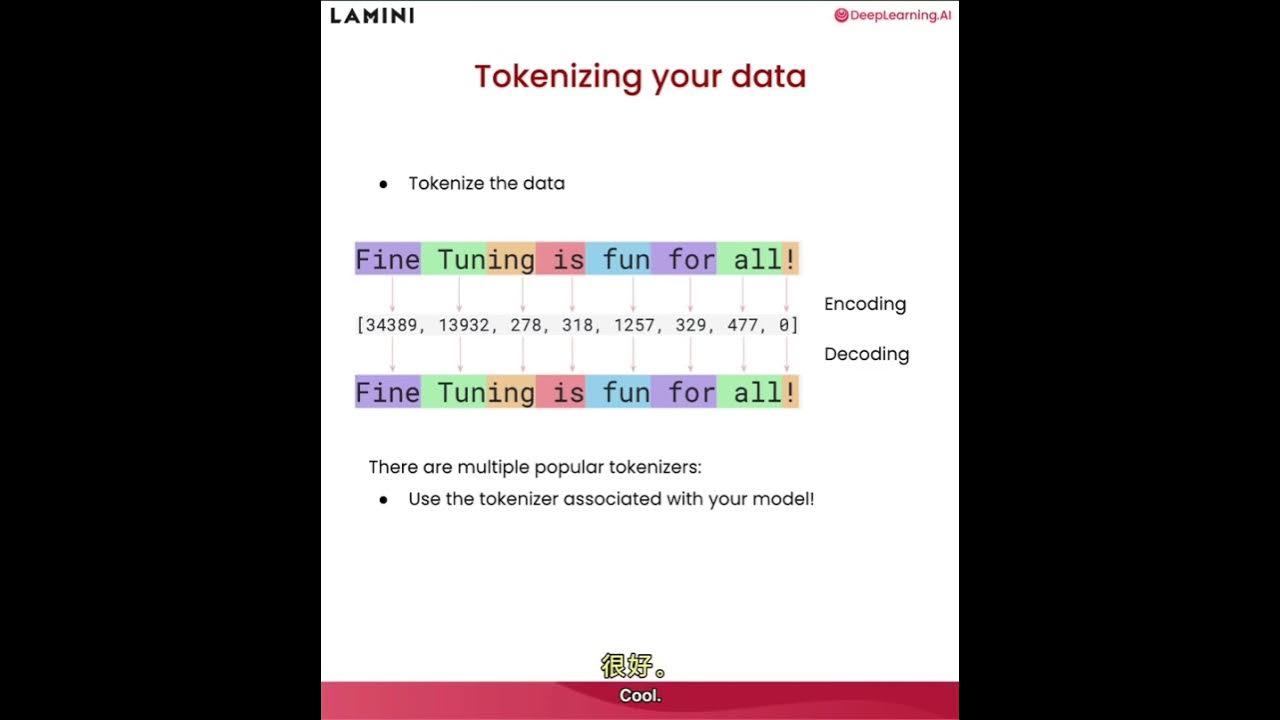
大语言模型微调之道5——准备数据

This AI Tool Will Make You a DATA ANALYST in Just 10 Minutes Step To Step Guide
5.0 / 5 (0 votes)
