Week 3 Lecture 13 Principal Components Regression
Summary
TLDRThis script delves into the concept of Singular Value Decomposition (SVD) and Principal Component Analysis (PCA) in the context of data analysis. It explains how SVD breaks down a matrix into diagonal entries and eigenvectors, and how PCA uses these components to find directions with maximum variance for data projection. The script highlights the benefits of PCA, such as reducing dimensionality while retaining significant variance, and discusses potential drawbacks, like ignoring the output variable when selecting principal components. It also touches on the importance of considering both input data and output variables for optimal feature selection in regression and classification tasks.
Takeaways
- 📊 The script discusses the concept of Singular Value Decomposition (SVD), where D is a diagonal matrix with eigenvalues or singular values, and V and U are matrices containing eigenvectors that span the column space of X.
- 🔍 Principal Component Analysis (PCA) is mentioned as a method that involves finding the covariance matrix of centered data and then performing an eigendecomposition to find principal component directions.
- 🌐 The principal component directions are orthogonal and each explains a certain amount of variance in the data, with the first principal component (V1) having the maximum variance.
- 📈 The script explains that projecting data onto the first principal component direction (V1) results in the highest variance among all possible projection directions, indicating the spread of data.
- 🔄 The process of PCA involves selecting principal components to perform regression, where each component is orthogonal and can be used independently in regression models.
- 📉 The script highlights that the first principal component direction minimizes the reconstruction error when only one coordinate is used to summarize the data.
- 📝 Principal Component Regression (PCR) is introduced as a method to perform regression using the selected principal components, with the regression coefficients being determined by regressing Y on the principal components.
- 🚫 A drawback of PCR is that it only considers the input data and not the output, which might lead to suboptimal directions if the output has specific characteristics.
- 📊 The script contrasts ideal PCA directions with those that might be more suitable for classification tasks, where considering the output can lead to better separating surfaces.
- 📉 The importance of considering both the input data and the output when deriving directions for tasks like classification is emphasized, as it can lead to more effective models.
- 🔑 The takeaways from the script highlight the mathematical foundations of PCA and its applications in feature selection and regression, as well as the importance of considering the output in certain contexts.
Q & A
What is the singular value decomposition (SVD) mentioned in the script?
-Singular Value Decomposition (SVD) is a factorization of a matrix into three matrices: D, a diagonal matrix with singular values on its diagonal; V, a P x P matrix with eigenvectors; and U, an N x P matrix that spans the column space of the original matrix X.
How is the covariance matrix related to the principal component analysis (PCA)?
-In PCA, the covariance matrix is derived from the centered data. The eigendecomposition of this covariance matrix provides the principal components, which are the directions of maximum variance in the data.
What are the principal component directions of X?
-The principal component directions of X are the columns of the V matrix obtained from the eigendecomposition of the covariance matrix of the centered data.
Why is the first principal component direction considered the best for projecting data?
-The first principal component direction is considered the best for projecting data because it captures the highest variance among all possible directions, resulting in the most spread-out data projection.
What is the significance of the orthogonality of principal components?
-Orthogonality of principal components means they are uncorrelated, allowing for independent regression analysis along each principal component direction, which can be useful for feature selection and data reconstruction.
How does the script relate the concept of variance to the principal components?
-The script explains that each principal component captures the maximum variance in its respective orthogonal space. The first principal component has the highest variance, followed by the second, and so on, with each subsequent component capturing the highest variance in the space orthogonal to the previously selected components.
What is the role of the intercept in principal component regression?
-In principal component regression, the intercept is the mean of the dependent variable (y-bar), which is added to the regression model to account for the central tendency of the data.
How does the script discuss the limitation of principal component regression?
-The script points out that principal component regression only considers the input data (X) and not the output, which might lead to suboptimal directions for regression if the output's characteristics are not taken into account.
What is the script's example illustrating the importance of considering the output in regression?
-The script uses a classification example where projecting data in the direction of maximum variance might mix different classes, leading to poor predictive performance. Instead, a direction that separates the classes clearly, even if it has lower variance, might be more beneficial for regression or classification.
How does the script suggest improving the selection of principal components for regression?
-The script suggests that considering the output data along with the input data might help in selecting better directions for regression, especially in cases where the output data has specific characteristics that could influence the choice of principal components.
What is the general process of feature selection using principal components?
-The general process involves selecting the first M principal components, performing univariate regression on each, and adding the outputs until the residual error becomes small enough, indicating a satisfactory fit.
Outlines

هذا القسم متوفر فقط للمشتركين. يرجى الترقية للوصول إلى هذه الميزة.
قم بالترقية الآنMindmap

هذا القسم متوفر فقط للمشتركين. يرجى الترقية للوصول إلى هذه الميزة.
قم بالترقية الآنKeywords

هذا القسم متوفر فقط للمشتركين. يرجى الترقية للوصول إلى هذه الميزة.
قم بالترقية الآنHighlights

هذا القسم متوفر فقط للمشتركين. يرجى الترقية للوصول إلى هذه الميزة.
قم بالترقية الآنTranscripts

هذا القسم متوفر فقط للمشتركين. يرجى الترقية للوصول إلى هذه الميزة.
قم بالترقية الآنتصفح المزيد من مقاطع الفيديو ذات الصلة
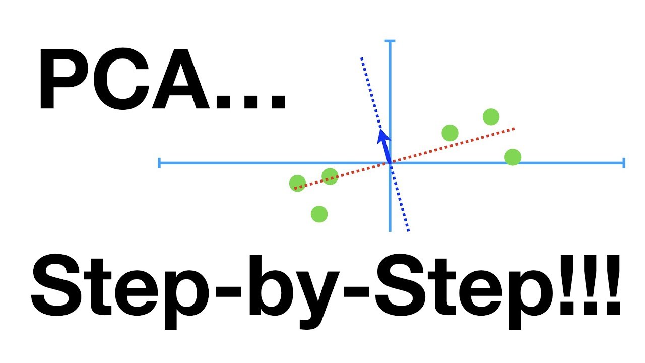
StatQuest: Principal Component Analysis (PCA), Step-by-Step
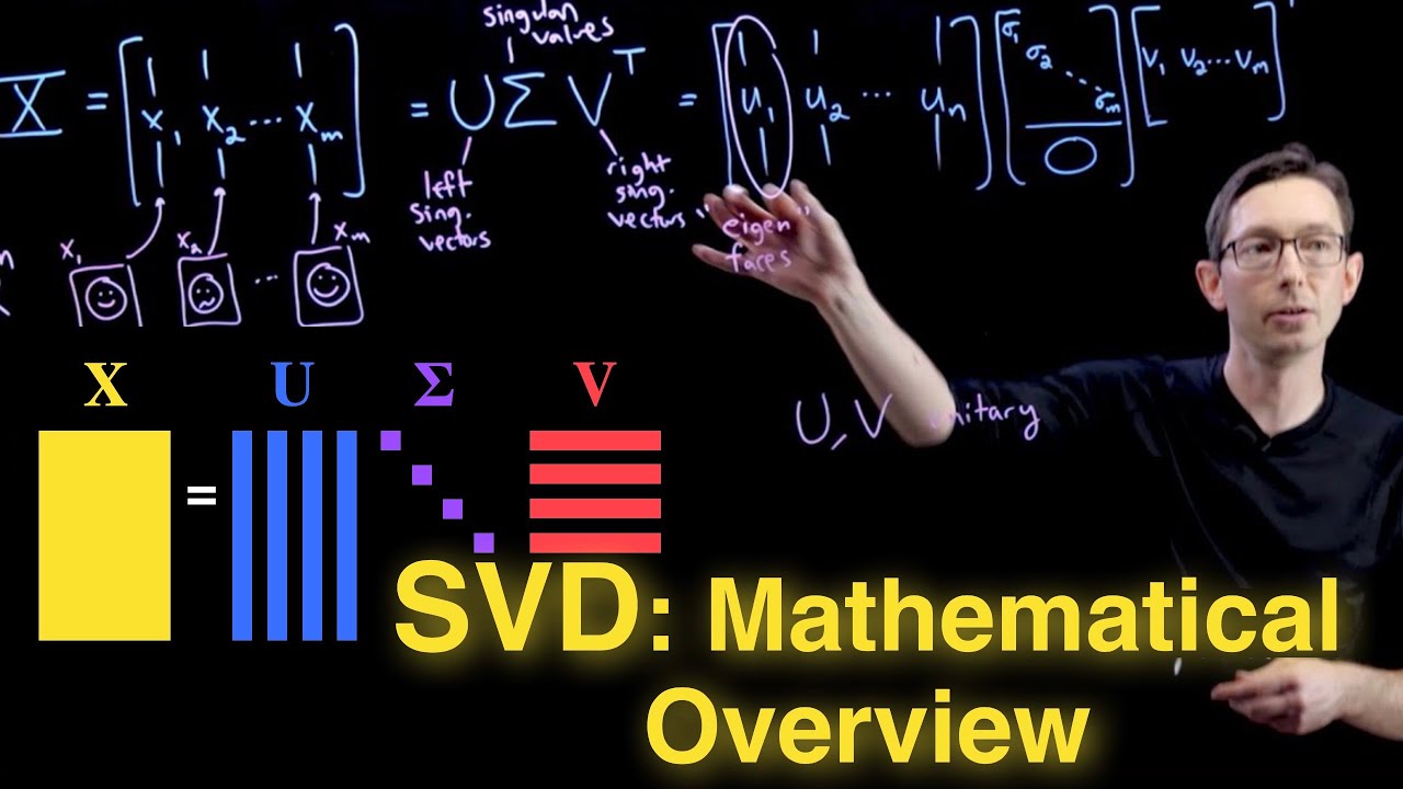
Singular Value Decomposition (SVD): Mathematical Overview

Pembahasan Analisis Komponen Utama (Part 1) | Review Konsep
PCA Algorithm | Principal Component Analysis Algorithm | PCA in Machine Learning by Mahesh Huddar
SINGULAR VALUE DECOMPOSITION (SVD)@VATAMBEDUSRAVANKUMAR

Image Compression with Python
5.0 / 5 (0 votes)
