Image Representation

Summary

In this lecture, the speaker transitions from discussing image formation to exploring how images are represented for processing through transformations. The lecture covers the reasoning behind using RGB color representation, the structure of the human eye, and various image operations such as point, local, and global transformations. Examples include image contrast adjustment and noise reduction. The speaker also touches on the complexity of these operations and introduces concepts like histogram equalization and Fourier transform, encouraging further reading and exploration.

Takeaways

• 👁️ RGB Representation: The human eye has three types of cones sensitive to specific wavelengths, corresponding to red, green, and blue, which is why images are represented in RGB despite the visible light spectrum being VIBGYOR.
• 🧬 Chromosomal Influence: The M and L cone sensitivities are linked to the X chromosome, leading to a higher likelihood of color blindness in males who have one X and one Y chromosome compared to females with two X chromosomes.
• 🐶 Animal Vision Variation: Different animals have varying numbers of cones, affecting their color perception; for example, night animals have one, dogs have two, and some creatures like mantis shrimp can have up to twelve different kinds of cones.
• 🖼️ Image as a Matrix: An image can be represented as a matrix, where each element corresponds to a pixel's intensity value, typically normalized between 0 and 1 or quantized to a byte (0-255).
• 🔢 Image Resolution: The size of the image matrix is determined by the image's resolution, which is captured by the image sensor.
• 📉 Image as a Function: An image can also be viewed as a function mapping from a coordinate location to an intensity value, aiding in performing operations on images more effectively.
• 🌗 Point Operations: These are pixel-level transformations that can adjust an image's appearance, such as brightness adjustment by adding a constant value to each pixel.
• 🔄 Local Operations: These consider a neighborhood of pixels around a coordinate to determine the output pixel's value, useful for noise reduction and smoothing.
• 🌍 Global Operations: The output pixel's value depends on the entire input image, with examples including Fourier transform and histogram equalization.
• 📈 Contrast Enhancement: Point operations like contrast reversal and contrast stretching can be used to enhance an image by manipulating pixel intensity values.
• 📊 Histogram Equalization: A method for contrast enhancement not covered in detail in the script, but mentioned as an important topic for further study.

Q & A

Why do we use RGB for representing images instead of VIBGYOR spectrum?

We use RGB color representation because the human eye has three kinds of cones that are sensitive to specific wavelengths corresponding to red, green, and blue. These cones do not peak exactly at red, green, and blue but at off colors in between, and for convenience, we use R, G, and B.

What are rods and cones in the human eye, and what is their function?

Rods are responsible for detecting the intensity of light in the environment, while cones are responsible for capturing colors. Humans have mainly three types of cones, each with specific sensitivities to different wavelengths.

Why are males more likely to be color-blind than females?

The M and L wavelengths, which are related to color perception, are stronger on the X chromosome. Since males have XY chromosomes and females have XX, males are more likely to be color-blind.

How does the number of cones in an animal's eye affect its color sensitivity?

Different animals have varying numbers of cones, which affects their color sensitivity. For example, night animals have 1 cone, dogs have 2, fish and birds have more, and mantis shrimp can have up to 12 different kinds of cones.

How is an image represented in a digital format?

An image can be represented as a matrix where each element corresponds to a pixel's intensity value. In practice, each pixel value ranges from 0 to 255, and these values are often normalized between 0 and 1 for processing.

What is the difference between a matrix and a function representation of an image?

A matrix is a discrete representation of an image, while a function represents the image in a continuous form. The function representation helps in performing operations on images more effectively.

How does the resolution of an image affect the size of its matrix representation?

The size of the matrix representation depends on the resolution of the image. Higher resolution images have larger matrices because they contain more pixels.

What are the three types of image operations, and how do they differ?

The three types of image operations are point operations, local operations, and global operations. Point operations affect a single pixel based on its value. Local operations consider a neighborhood of pixels around a point. Global operations depend on the entire image.

How can point operations be used to reduce noise in an image?

Point operations alone cannot effectively reduce noise. However, by taking multiple images of a still scene and averaging them, noise can be mitigated to some extent due to the averaging process.

What is the formula for linear contrast stretching, and how does it work?

The formula for linear contrast stretching is to take the original pixel value, subtract the minimum intensity (I_min), multiply by a ratio (I_max - I_min) / (max(I) - min(I)), and then add I_min. This stretches the contrast to use the full range of pixel values.

Can you provide an example of a local operation used for noise reduction?

A moving average is an example of a local operation used for noise reduction. It involves taking the average of pixel values within a neighborhood around a point to smooth out noise.

What is the difference between local and global operations in terms of computational complexity?

The computational complexity for a point operation is constant per pixel. For a local operation, it is proportional to the square of the neighborhood size (p^2). For a global operation, the complexity per pixel is proportional to the square of the image size (N^2).

What is histogram equalization, and why is it used in image processing?

Histogram equalization is a method used to improve the contrast of an image by redistributing its intensity values. It is used to stretch the contrast to cover the full range of intensity values, making the image appear more vivid.

Outlines

00:00

👀 Human Vision and Image Representation

This paragraph discusses the human eye's structure and its relation to color representation in images. It explains that the visible light spectrum is not directly represented as VIBGYOR due to the presence of three types of cones in the human eye, which are sensitive to specific wavelengths corresponding to red, green, and blue. This is why the RGB color model is used. The paragraph also touches on the fact that color blindness is more common in males due to the X-chromosome linkage of the M and L cones. It further explores the diversity of color perception in nature, mentioning that different animals have varying numbers of cones, from one in night animals to up to twelve in mantis shrimps. The paragraph concludes with an introduction to image representation as matrices, explaining how images can be normalized and the significance of image resolution on matrix size.

05:01

📚 Image Representation and Transformations

The second paragraph delves into how images are represented and transformed. It begins by describing images as matrices or functions, with the function mapping from a coordinate location to an intensity value. The paragraph explains the concept of digital images as discrete and quantized versions of continuous functions, highlighting the process of sampling and quantization. It then discusses image transformations, providing examples of point operations such as adding a constant to lighten an image and reflecting an image around the vertical axis. The paragraph introduces the three types of image operations: point, local, and global, explaining their differences and complexities. It also touches on image enhancement techniques like contrast reversal and contrast stretching, illustrating these with examples and formulas.

10:07

🔍 Point Operations and Their Limitations

This paragraph examines point operations in image processing, which affect a single pixel based on its intensity alone. It discusses the limitations of point operations, such as their inability to fully account for the complexities of image formation influenced by factors like light source, surface geometry, and sensor capture. The paragraph provides an example of noise reduction in images, suggesting that averaging multiple images of a still scene can mitigate noise. However, it acknowledges the impracticality of this method due to the constant motion in scenes and the difficulty of obtaining multiple images.

15:10

🌟 Transition to Local Operations for Noise Reduction

The fourth paragraph transitions from point operations to local operations, which consider the neighborhood of pixels around a given coordinate when processing an image. It uses the example of a moving average to illustrate local operations, demonstrating how a 3x3 window can be used to average pixel values and smooth out noise in an image. The paragraph explains the process of moving the window across the image and calculating the average for each position, resulting in a smoother output image. It also provides the formula for the moving average operation, emphasizing its role in local image processing.

20:10

🌐 Global Operations and Fourier Transform

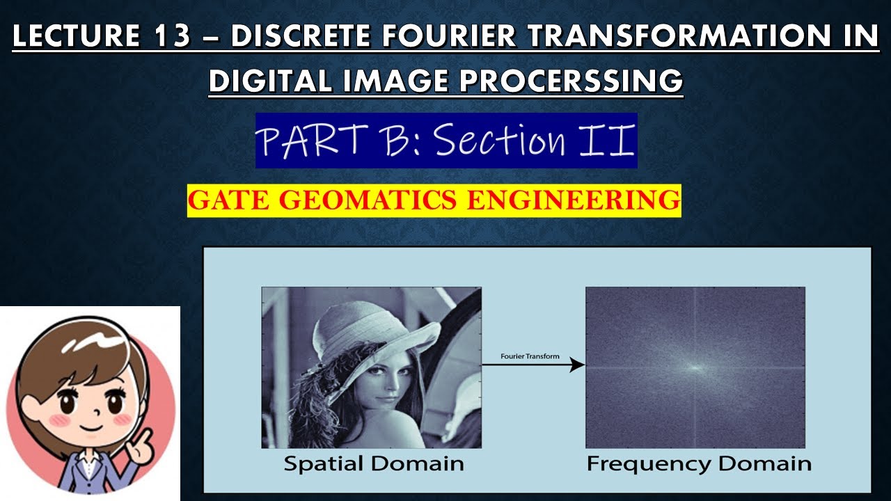
The final paragraph introduces global operations in image processing, where the value of a pixel in the output image depends on the entire input image. It provides the example of the Fourier transform, which will be discussed in more detail in later lectures. The paragraph also mentions other global operations that may depend on different applications. The lecture concludes with a reading assignment from Szeliski's book and encourages students to explore histogram equalization, a technique for improving the contrast in images.

Keywords

💡Image Representation

Image Representation refers to the method of encoding and storing visual information in a digital format. In the context of the video, it is the foundation for image processing and transformations. The script explains that an image can be represented as a matrix, where each element corresponds to a pixel's color intensity, and also as a function, which allows for more effective operations on images. The video emphasizes the importance of understanding how images are represented to effectively manipulate and analyze them.

💡RGB Color Model

The RGB color model is a method of representing colors in digital imaging, where the intensity of red, green, and blue light are combined to produce a wide array of colors. The script delves into why RGB is used instead of the visible light spectrum VIBGYOR, explaining that the human eye has three types of cones sensitive to specific wavelengths close to red, green, and blue, which is why these colors are fundamental in digital image representation.

💡Cones

Cones are photoreceptor cells in the retina that are responsible for detecting color. The script mentions that the human eye has three types of cones, each sensitive to different wavelengths, corresponding to red, green, and blue light. This sensitivity is crucial for the RGB color model used in digital imaging and is a key concept in understanding color perception and image processing.

💡Color Blindness

Color blindness is a condition where an individual cannot perceive some or all color differences in the spectrum. The script touches on the genetic aspect of color blindness, noting that the M and L cones, which are responsible for color perception, are stronger on the X chromosome. This implies that males, having only one X chromosome, are more likely to be color-blind, which is a significant point in the discussion of color perception and its biological underpinnings.

💡Matrix

In the context of image processing, a matrix is a two-dimensional array of numbers used to represent an image, where each number corresponds to the intensity of a pixel. The script uses the matrix as an example to illustrate how an image can be broken down into its constituent parts for processing. This concept is fundamental to understanding how images are manipulated at a pixel level.

💡Normalization

Normalization in image processing refers to the process of scaling pixel values to a specific range, typically between 0 and 1, to facilitate image analysis and processing. The script mentions that in practice, pixel values range from 0 to 255, but are often normalized for certain operations. This is important for ensuring consistency and comparability across different images and processing techniques.

💡Point Operations

Point operations are image processing techniques where the value of a pixel in the output image depends solely on the corresponding pixel in the input image. The script provides examples of point operations, such as adjusting brightness by adding a constant value to each pixel. These operations are simple and fast but may not capture the full complexity of an image, as they do not consider the context of neighboring pixels.

💡Local Operations

Local operations are a type of image processing where the value of a pixel in the output image is determined by considering a neighborhood of pixels around the corresponding location in the input image. The script describes an example of a moving average, which smooths out noise by averaging pixel values within a local region. This approach is useful for noise reduction and blurring, as it takes into account the spatial context of each pixel.

💡Global Operations

Global operations affect the entire image, with each pixel's value in the output image depending on the entire input image. The script mentions Fourier transform as an example of a global operation, which is used for frequency domain analysis. These operations are more complex and computationally intensive but can reveal properties of the image that are not apparent in point or local operations.

💡Histogram Equalization

Histogram equalization is an image processing technique used to improve the contrast of an image by redistributing its intensity values. The script suggests this as a homework topic, indicating that it is a method for adjusting the distribution of pixel intensities to enhance the visibility of image details. This technique is particularly useful for images with poor contrast, as it can help to spread out the pixel values more evenly across the intensity range.

💡Noise Reduction

Noise reduction is the process of minimizing random variations of brightness or color in an image, which can be caused by various factors such as sensor noise or dust on the lens. The script discusses the limitations of point operations for noise reduction and suggests that averaging multiple images can help to mitigate noise. This is an important concept in image processing, as it relates to image quality and the reliability of subsequent analysis.

Highlights

Introduction to the representation of images for processing using transformations.

Explanation of the RGB color representation based on the human eye's sensitivity to specific wavelengths.

The human eye has three kinds of cones, corresponding to S, M, and L sensitivities, which relate to red, green, and blue.

Males are more likely to be color-blind due to the M and L wavelengths being stronger on the X chromosome.

Diversity in color perception across different species, from 1 cone in night animals to 12 in mantis shrimp.

Images can be represented as matrices, with values normalized between 0 and 1 or 0 and 255.

Each color channel in an image has its own matrix, and the size depends on the image resolution.

Images can also be represented as functions, facilitating more effective operations on images.

Digital images are discrete, sampled, and quantized versions of continuous functions.

Point operations on images are defined, where the output pixel depends only on the corresponding input pixel.

Example of a point operation: Adjusting image brightness by adding a constant value to each pixel.

Local operations consider a neighborhood of pixels around a coordinate, unlike point operations.

Global operations depend on the entire input image for the value of a single output pixel.

Complexity analysis of point, local, and global operations in terms of per-pixel calculations.

Point operation example: Contrast reversal, where the output pixel is the maximum intensity minus the input pixel value.

Contrast stretching explained, a method to utilize the full range of pixel values to enhance image contrast.

Introduction to histogram equalization as a technique for contrast enhancement.

Limitations of point operations in handling image noise, especially in dynamic scenes.

Local operation example: Moving average to reduce noise by averaging pixel values in a neighborhood.

Global operations like Fourier transform are mentioned as examples that depend on the whole image.

Assignment on reading Szeliski's book chapter 3.1 and understanding histogram equalization.

Transcripts

In last lecture we spoke about image  formation and now we will move on to  

how do you represent an image so you  can process it using transformations.

So, we did leave one question during the last  lecture which is if the visible lights spectrum  

is VIBGYOR from violet to red, why do  we use an RGB colour representation,  

hope you all had a chance to think  about it, read about it and figure out  

the answer. The answer is the human  eye is made up of rods and cones.

The rods are responsible for detecting the  intensity in the world around us and the cones  

are responsible for capturing the colours and  it happens that the human eye there are mainly  

three kinds of cones and these cones has specific  sensitivities and the sensitivities of these cones  

are at specific wavelengths which are represented  by S, M and L on this particular figure.

So, if you look at where these cones  peak at that happens to be close to red,  

green and blue and that is the reason  for representing images as red,  

green and blue in all honesty the peaking  does not happen exactly red, green and blue,  

it actually happens in off colours in between  but for convenience we just use R, G and B.

Some interesting facts here it happens  that the M and L wavelengths here are  

stronger on the X chromosome, so which  means males who have the XY chromosome,  

females have the XX are more likely to  be color-blind. So, also it is not that  

all animals have the same three cones while  humans have 3 cones, night animals have 1 cone,  

dogs have 2 cones fish and birds have more colour  sensitivity and it goes to 4, 5 or in a mantis  

shrimp goes up to 12 different kinds of cones. So,  nature has abundance of how colours are perceived.

Moving on to how an image is represented, the  simplest way to represent an image which you  

may have already thought of is to represent an  image as a matrix. So, here is the picture of the  

Charminar and if you look at one small portion  of the image the clock part you can clearly see  

that you can zoom into it and you can probably  represent it as a matrix of values in this case  

line between 0 and 1 and obviously you will have  a similar matrix for the rest of the image too.

So, but is very very common in practice while  we are talking here about using it with values  

0 to 1, in practice people use up to a byte for  representing each pixel which means every pixel  

has can take a value between 0 and 255 to byte  and a in practice we also normalize these values  

between 0 and 1 and that is the reason why you  see these kinds of values in a representation.

And also, to keep in mind is that for every colour  channel you would have one such matrix if you  

had a Red, Green, Blue image, you would have one  matrix for each of these channels. What would be  

the size of this matrix, the size of these matrix  would depend on the resolution of the image. So,  

recall again what we spoke about the image  sensing component in the last lecture,  

so depending on what resolution the  image sensor captures the image in,  

that would decide the resolution  and hence the size of the matrix.

A matrix is not the only way to represent  an image, an image can also be represented  

as a function, why so? It just helps us have  operations on images more effectively if we  

represent it also as a function, certain  operations at least. So, in this case we  

could talk about this function being going from R  square to R, where R square simply corresponds to  

one particular coordinate location on the image  say i, j and that is what we mean by R square.

And the range R is the intensity of the image  that could assume a value between 0 to 255 or  

0 to 1 if you choose to normalize the image.  And a digital image is a discrete a sampled  

quantized version of that continuous function  that we just spoke about, why is it a sample  

quantized version by sample we mean that we  sample it at that resolution, originally the  

function can be continues which is like the  real world in which the image was captured.

Then we sample the real world at some particular  pixel values on some grid with respect to a point  

of reference and that is what we call as a  sample discrete version of the original of  

the original continuous function. Why quantized  because we are saying that the intensity can be  

represented only as values between 0 and  255 and also in the same steps you cannot  

have a value 0.5 for instance at least in this  particular example. Obviously you can change it  

if you like in a particular capture setting but  when we talk about using a byte for representing  

a pixel you can only have 0, 1, 2 so on and  so forth till 255 you can not have a 0.5 so  

you actually discretized or you have quantized  the intensity value that you have in the image.

So, let us talk about transforming images when we  look at them as functions, so here is an example  

transformation so you have a face and we seem  to have lighten the face in some way. What do  

you think is the transformation here?  Can you guess? In case you have not,  

the transformation here is if your input image  was I and your output image was I hat you can  

say that I hat is I(x,y) plus 20. And 20 is  just a number if you want it to be more lighter  

you would say plus 30 or plus 40, again here we  assuming that the values lie between 0 and 255.

One more example, let say this is the  next example where on the left you have  

a source image on the right you have  a target image. What do you think is  

the transformation, the transformation  is y hat of xy would be I of minus x,  

y the image is reflected around the vertical  axis, y axis is fixed and then you rotate,  

you flip the x axis values. If you notice here  both of these examples, the transformations  

happen point wise or pixel wise, in both these  cases we have defined the transformation at a  

pixel level. Is that the only way you can  perform a transformation? Not necessarily.

Very broadly speaking we have three  different kinds of operations that  

you can perform on an image you have  point operations, point operations are  

what we have just spoken about where a  pixel at the output depends only on that  

particular pixel the same coordinate location  in the input that would be a point operation.

A local operation is where a pixel at  the output depends on an entire region  

or neighbourhood around that coordinate in  the input image, and a global operation is  

one in which the value that a pixel assumes in  the output image depends on the entire input,  

on the entire input image. In terms  of complexity for a point operation  

the complexity per pixel would just be  a constant, for a local operation the  

complexity per pixel would be p square assuming  a pxp neighbourhood, local neighbourhood around  

the coordinate that you considering for that  operation. And in case of global operations  

obviously the complexity per pixel will  be N square where the image is N cross N.

Let see a couple of more point operations  and then we see local and global,  

so here is a very popular point operation  that you may have used in your smartphone  

camera or adobe photoshop or any other task  image editing task that you took on. It is an  

image enhancement task and we want to reverse  the contrast, reversing the contrast we want  

the black to become white and the dark grey  to become light grey so on and so forth.

What do you think? How would you implement this  operation? In case you have not worked it out yet,  

the operation would be at a particular pixel  is a point operation so at particular pixel m  

naught n naught your output will be I max minus  the original pixel at that location plus I min,  

you are flipping so if you had a value say 240  which is close to white generally white is to 255  

and 0 is black if you had a value 240, now that  is going to become 15 because I max in our case is  

255 and I min is 0. I min is 0, I min obviously  does not matter but this formula is assuming  

at more general setting where I min could be  some other values that you have in practice.

Moving on let us take one more example of image  enhancement again, but this time you are going  

to talk about stretching the contrast when we  stretch the contrast, you are taking the set  

of values and you are stretching it to use the  entire set of values that each pixel can occupy,  

so you can see here this is again a very common  operation that you have used if you edited images.

What do you think is the operation here this is  slightly more complicated then the previous one,  

in case you already do not have the  answer, remember let us first find  

out the ratio so you have a typical I max  minus I min which is 255 minus 0 by max of  

I in this image minus min of I in this  image let us assume hypothetically that  

this image on the left had its max value  to be 200 and its min value to be 100.

If that is the case this entire ratio here that  you see is going to become 2.55 this is 255 minus  

0 divided by 100. 200 minus 100 which will be  2.55. So, you are simply saying that I am going to  

take the original pixel whatever let us assume for  the moment that the original pixel had a value,  

say 150 so if this had the value 150 so you  subtracting a minimum, so which means you  

have a value the minimum is 100, so you are  going to have 50 into 2.55 plus I min for us  

which is 0 which roughly comes to 128. So  that is 50 percent of the overall output.

So, what was 150 which was in the middle of the  spectrum in the range of values that we had for  

this input image now becomes 128 which becomes  the middle of the spectrum for the entire set  

of values between 0 to 255, you are simply trying  to stretch the contrast that you have to use all  

the values that you have between 0 and 255. Which  means what would have gone from dark grey to light  

grey now goes from black to white that is how  you increase a contrast, so this is called linear  

contrast stretching a simple operation again but  in practice we do something more complicated.

So, we do what is known as histogram  equalization you may have again heard  

about it perhaps used it in certain  settings if you have heard about it,  

read about it and that is going to be  your homework for this particular lecture.

So, let ask the question do  point operations satisfy all  

the requirements we have of operating on  images? Let us take one particular example,  

so we know that a single points intensities  influence by multiple factors we talked about  

at the last time and it may not tell us everything  so because it influence by light source strength,  

direction, surface geometry, sensor  capture, image representation and so on.

So, it may not be fully informative so  let us take an example to show this,  

so let us assume we give you a camera and  you have a still scene no movement how do  

you reduce noise using point operations. The  noise could be cause by some dust blowing in  

the scene could be cause by speck of dust  on the lens of your camera or by any other  

reason for that matter could that they  could be a damage on one of the sensors.

Noise could be at several, at various levels,  how would you reduce noise using only point  

operations? The answer you have to take  many images and average them because it  

is still scene, we can keep taking images  and hope that the noise gets averaged out,  

across all of your images that you took  and you take the average of all of your  

images it is a bunch of matrices you can  simply taken element wise average of all  

of those matrices and that can help you  mitigate the issue of noise to some extent.

But clearly that is the stretch you do not  get multiple images for every scene all  

the time and you do not get a still scene  that is absolutely still all the time to  

there is always some motion and so this may not  be a method that works very well in practice. So,  

to do this we have to graduate from  point operations to local operations.

So, let see what a local operation means,  

as we already said a pixel value at output  depends on an entire neighbourhood of pixels  

in the input around that coordinate whichever  coordinate we want to evaluate the output at.

So, here is a very simple example to understand  what local operation is standard example is what  

is known as the moving average, so here you have  the original input image I as you can see the  

input image I is simply a white box placed  on a dark grey background or in this case a  

black background because you can see zeros as the  values assume that that means a black background.

So, the image has the particular resolution  in this particular case it is a 10 cross 10  

image and the white box is located in a  particular region. But the problem for  

us is we are going to assume that this  black pixel in the middle here and this  

white pixel here are noise pixels that came  in inadvertently. So, how do you remove them?

So, the way we going to remove them is to consider  a moving average, so you take a 3 cross 3 window,  

need not be 3 cross 3 all the time could be a  different size, further moment we are going to  

take it 3 cross 3 and simply take the average  of the pixels in that particular region. So,  

the average here comes out to be 0, so you  fill it at the center location of that box.

Moving on you now move the 3 cross 3 box to  the next location you again take an average  

now the sum turns out be 90, 90 by 9, 10.  Similarly, move the box slide the box till  

further and once again take the average of all  pixels in the box in the input and that gives  

you one value in the output. Clearly you can see  that this is a local operation, the output pixel  

depends on a local neighbourhood around the  same coordinate location in the input image.

And you can continue this process and you  finally will end up creating the entire image  

looking somewhat like this, so you can see now  you may have to squint your eyes to see this,  

you can see now that the seemingly  noise pixels here and here in the  

input have been smoothened out because  of the values of the neighbours and the  

output looks much smoother, here is a low  resolution image so it looks a bit blocky.

But if you have higher resolution it  would look much smoother to your eyes. So,  

what is the operation that we did, let us  try to write out what operation we did. So,  

we said here that I hat at a particular location  say x,y is going to be, you are going to take a  

neighbourhood. So, which means you going  to take the same location in your input  

image and say you are going to go from say x  minus some window k to x plus some window k.

Similarly, we are going to go from some y  minus k to y plus k and let us call this say i,  

let us call this say j you are going to  take the values of all those pixels in  

the input image. And obviously we  are going to average all of them,  

so you are going to multiply this entire  value by 1 by because the neighbourhood  

goes from x minus k to x plus k there  are totally 2 k plus 1 pixels there.

So, you are going to have 2k plus 1 square,  because for x will have 2k plus 1 pixels,  

for y you will have 2k plus 1 pixels and  then you just, so the total number of pixels  

is going to be 1 cross the other and in this  particular example that we saw k was 1 for us,  

we went from x minus 1 to x plus 1, so if  you took a particular location on the output,  

you took the corresponding location on the input  and then one to the left and one to the right. So,  

from x minus 1 to x plus 1, y minus 1 to y  plus 1 and that creates a 3 cross 3 matrix  

for you and that is what we going to finally  normalize it by. That becomes the operation  

that you have for your moving average, so  this is an example of a local operation.

Moving to the last kind of an operation called  a global operation as we already mentioned in  

this case the value at the output pixel depends on  the entire input image. Can you think of examples?

In case you have already not figured out,  a strong example of something like this,  

this what is known as a Fourier transform we will  see this in a slightly later lecture but there are  

other operations to that can be global depending  on different applications, we will see more of  

this a bit later and we will specifically  talk about Fourier transform a bit later.

That is about this lecture so your readings  are going to be chapter 3.1 of Szeliski s  

book and also as we mentioned think about the  question and read about histogram equalization  

and try to find out how it works and what is the  expression you would write out to make it work.