Control Systems Lectures - Time and Frequency Domain
Summary
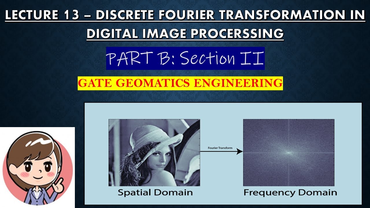
TLDRThis lecture introduces the concepts of time domain and frequency domain, emphasizing their physical meaning and applications. It begins with familiar time-related equations, like distance as a function of velocity and time. The lecture then explores harmonic oscillators, showing how sinusoidal motion can be described in the time domain and its corresponding frequency domain representation. Key topics include Fourier series and transform, which convert time domain signals into frequency domain representations, and Laplace transforms, used for analyzing systems with exponential growth or decay, helping solve differential equations in physics and control system design.
Takeaways
- 😀 Time domain equations are intuitive because they reflect familiar concepts like time, velocity, and acceleration.
- 📈 Distance is a function of time and velocity, easily visualized through equations like D = V × T.
- 🌀 A harmonic oscillator follows a sinusoidal motion that can be represented mathematically, and its force is negatively proportional to the distance from the neutral point.
- ⚖️ Newton's second law is used to describe the motion of a mass attached to a spring, leading to a sinusoidal solution in the time domain.
- 🎶 Fourier series allows for the transformation of a repeating time-domain signal into the frequency domain, expressed as an infinite summation of sinusoids.
- 🎸 Combining sinusoids of different frequencies creates complex time-domain signals that can be plotted in the frequency domain.
- 🔄 The Fourier transform extends the Fourier series to non-repeating signals, representing any signal as a summation of sinusoids with frequency, amplitude, and phase.
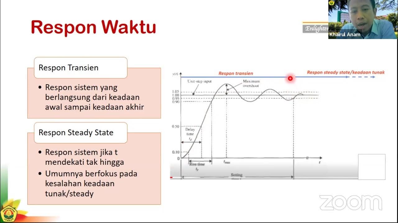
- 📉 Adding damping to an oscillator introduces an exponential decay term, which adjusts the time-domain response.
- 🧮 The Laplace transform extends the Fourier transform by accounting for exponential growth and decay, transforming signals into the S-domain for easier differential equation solving.
- 🔧 The S-domain is useful for control system design, offering insights into stability margins and simplifying complex time-domain calculations.
Q & A
What is the difference between time domain and frequency domain?
-The time domain represents how a signal or physical quantity changes over time, while the frequency domain represents the signal's composition in terms of its frequencies. Time domain equations are often intuitive as they relate to physical concepts like velocity and distance, while the frequency domain helps in analyzing the periodic or harmonic components of a signal.
What is a harmonic oscillator, and how is it described in the time domain?
-A harmonic oscillator is a system where the restoring force is proportional to the displacement, such as a spring with a mass attached. In the time domain, its motion can be described by a sinusoidal function representing how the displacement varies over time.
How does Newton's second law apply to the harmonic oscillator?
-In the harmonic oscillator, Newton's second law states that the force acting on the mass is equal to its mass times acceleration (F = ma). The restoring force is proportional to the displacement (F = -kx), leading to a differential equation that describes the sinusoidal motion of the system.
What is the purpose of the Fourier transform in signal analysis?
-The Fourier transform is used to represent a time-domain signal in the frequency domain. It expresses the signal as a sum of sinusoids at different frequencies, amplitudes, and phases, providing insight into the signal's frequency content.
What is the difference between a Fourier series and a Fourier transform?
-A Fourier series represents a periodic time-domain signal as a sum of sinusoids at discrete harmonic frequencies. In contrast, the Fourier transform generalizes this concept to non-periodic signals, representing them as a continuous spectrum of frequencies.
How does damping affect the motion of a harmonic oscillator, and how is it represented mathematically?
-Damping causes the amplitude of the harmonic oscillator's motion to decrease over time due to energy loss, usually to friction or resistance. Mathematically, this is represented by an exponential decay term in the time domain, modifying the simple sinusoidal motion.
Why is phase important in the frequency domain representation of a signal?
-Phase determines the position of the sinusoidal components relative to each other in time. In control systems, phase is crucial because it can affect system stability and performance, even when the amplitude and frequency content are known.
What is the significance of Joseph Fourier's work in signal processing?
-Joseph Fourier showed that any periodic time-domain signal can be represented as a sum of sinusoids at different frequencies. This principle forms the basis of the Fourier series and Fourier transform, which are essential tools for analyzing signals in the frequency domain.
What is the purpose of the Laplace transform, and how does it differ from the Fourier transform?
-The Laplace transform is used to analyze systems that exhibit exponential growth or decay in addition to sinusoidal behavior. It extends the Fourier transform by including a real component (σ), which captures exponential behavior, making it useful for solving differential equations in control systems and other physical applications.
How is stability margin quantified in control system design using the S-plane?
-Stability margin in control systems is quantified using the S-plane, where the system's poles and zeros are mapped. The distance of the poles from the imaginary axis indicates the stability of the system. Systems with poles closer to the left half of the S-plane are more stable.
Outlines
⏳ Introduction to Time and Frequency Domains
This paragraph introduces the concepts of time domain and frequency domain. It begins by explaining the physical meaning of time domain equations, such as how distance is a function of velocity and time. A real-world example is given, describing a journey to meet someone by walking a specific distance within a set time. The paragraph then shifts to a harmonic oscillator example, explaining the linear relationship between force and distance in a spring system. The motion of a mass attached to a spring is described using Newton's second law, which leads to the derivation of a sinusoidal motion equation in the time domain. The transition from time domain to frequency domain is then mentioned, focusing on how a pure sinusoid is represented by a single frequency in the frequency domain.
📊 Fourier Series and Frequency Representation
This section discusses the mathematical approach to representing signals in the frequency domain, introducing the Fourier series, which can decompose any periodic signal into a sum of sinusoids. Joseph Fourier's 1807 equation is mentioned, explaining that any repeating signal can be represented by a series of sinusoids at increasing frequencies. The paragraph explains how the frequency domain representation of a signal changes as the period increases, leading to a continuous frequency spectrum in non-repeating signals. This forms the basis of the Fourier transform, which transforms time-domain signals into frequency-domain representations. The Fourier transform can be applied to any signal, capturing its frequency, amplitude, and phase.
🔄 Fourier Transform and Real-World Applications
The final paragraph touches upon the broader utility of the Fourier transform and how it leads to the Laplace transform for more complex physical systems. While the Fourier transform helps analyze the frequency content of a signal, it falls short in scenarios involving differential equations with exponential terms, such as systems with damping. The introduction of the Laplace transform, which incorporates both the frequency and exponential components, allows for more comprehensive analysis. This paragraph briefly introduces the S-domain, explaining how the Laplace transform aids in solving differential equations and control system design by simplifying complex time-domain convolutions into algebraic expressions in the S-plane. The paragraph concludes by stating that future lessons will delve deeper into the Laplace transform.
Mindmap
Keywords
💡Time Domain
💡Frequency Domain
💡Harmonic Oscillator
💡Restoring Force
💡Fourier Transform
💡Sine Wave
💡Laplace Transform
💡Damping
💡Newton's Second Law
💡Sinusoidal Function
Highlights
Introduction to the time domain and frequency domain.
Understanding physical meaning of time domain equations using algebraic variables like time, velocity, and acceleration.
Example of distance as a function of time, illustrating travel and arrival over time.
Explanation of harmonic oscillator and its relationship with springs and restoring force.
Mathematical description of motion in time domain using Newton’s second law.
Introduction to frequency domain representation of sinusoidal functions.
Description of amplitude and frequency representation in the frequency domain.
Discussion on Fourier series and its role in transforming time domain signals into frequency domain.
Example of superposition of two sinusoidal signals and its representation in both time and frequency domains.
Introduction to Joseph Fourier’s work on representing periodic signals through infinite summation of sinusoids.
Explanation of harmonic frequencies and their role in forming complex waveforms like sawtooth waves.
Introduction to Fourier transform, its role in representing both repeating and non-repeating signals.
Introduction to exponential terms and damping effects in systems with energy loss.
Transition from Fourier transform to Laplace transform for solving differential equations and including exponential decay.
Introduction to the S-domain and its importance for analyzing system stability and control design.
Transcripts
this lecture is an introduction to time
domain and frequency domain it's easy to
see the physical meaning of time domain
equations because most likely you have
been using algebraic variables to
represent concepts like time velocity
and acceleration for many years distance
equals velocity times time or in other
words how far you travel D is related to
how fast you are going V times how long
you are traveling for T this can also be
said D is a function of V and T say for
example when you want to meet someone
for dinner in three hours at their house
which is a distance D from you you start
walking in a straight line and after one
hour you've made it a third of the way
another hour passes and another third of
the distance passes so that after three
hours you arrive at the house right on
time although you've walked in a
straight line and therefore in a single
dimension in your perspective you've
also passed through time which can be
thought of as a second dimension in this
case and if we cross plot the dependent
variable distance in the independent
variable time we can get a relationship
between how your distance has changed
with time or another way of saying that
is that distance is a function of time
let's try this again and this time let's
use a simple harmonic oscillator say you
were able to design a spring that had
these unique characteristics every time
you doubled the stretched distance of
the spring the restoring force also
doubled so in this case the neutral
distance is x equals zero the stretched
distance is x equals one and it produces
a restoring force F if you stretch the
spring to X equal two the restoring
force also doubles similarly when you
compress the spring by the same distance
that you stretched it the force will be
equal and opposite so again if you
compress the spring to x equals minus
one you'll have a positive restoring
force F x equals minus two and you'll
have a positive restoring force to
in other words you've designed a linear
spring in which the force is negatively
proportional to the distance from the
neutral point if we attach a mass M to
the end of the spring and then we set
the mass in motion by hitting it with a
hammer
that is we impart an impulse into the
system which corresponds to
instantaneous velocity we can observe
the resulting motion over time and if
you're familiar with the motion of the
jack in the box after it pops out of the
box you'll recognize a familiar bobbing
motion that might resemble a sinusoid
now mathematically we can describe the
motion of this system in the time domain
using Newton's second law a free body
diagram of the mass shows that the only
force acting on it is the restoring
force from the spring minus K times X
and we can set that equal to the inertia
of the system which is mass times
acceleration or mass times x double-dot
rearranging this equation produces a
differential equation that describes the
motion of this system it can be shown
that the general solution of this
differential equation is truly a
sinusoid in the form the amplitude times
the sine of the natural frequency times
time plus the phase this is the
description of the resulting motion in
the time domain but how would you
describe this in the frequency domain
since this is a pure sinusoidal the
resulting frequency domain
representation is straightforward we can
plot the amplitude and frequencies
across the spectrum of the sinusoids
that make up the signal so in this case
we have a single peak at frequency 2 pi
Omega with a height corresponding to
amplitude a the rest of the spectrum
would have zero amplitude often phase is
discarded with this representation and
only amplitude and frequency are looked
at however as it will become obvious in
later lessons phase is crucial in
designing a control system now that we
understand a pure sinusoidal the
frequency domain the next question is
how to represent a more complex time
domain signal or function in the
frequency domain
if we take two sinusoidal sum them
together we can create a signal that is
a superposition of the two frequencies
and the resulting waveform would have
two frequency inputs with corresponding
amplitudes in this example the signal on
the Left has amplitude ay-one with a
period t1 and the signal in the middle
has an amplitude ay-two with period t2
if we plot this against frequency or one
over the period you would see two
distinct frequencies with two separate
amplitudes as you'd expect now these two
representations the time and the
frequency representation are both
equivalent mathematician Joseph Fourier
in 1807 published an equation that
stated that if you have a signal that
repeats over the period T or the
frequency of the repeating pattern is 1
over T that that time domain signal can
be represented by an infinite summation
of sinusoids at ever increasing
frequencies the equation is a bit too
long to write down here and I don't want
to go too far into the math in this
lecture so I will just say that a
Fourier series will transform it from
the time domain on the left to the
frequency domain on the right even
though this is a summation of infinite
number of frequencies not every
frequency as possible the key here is
that each sinusoidal of the lowest
frequency usually called the first
harmonic and then by multiplying the
first harmonic frequency by an integer
in you can get the second third and
fourth harmonic frequencies and so on
all the way up to infinity
for example this sawtooth wave input
does not look anything like the smooth
contours of the sine wave
yet by adding an infinite series of
these harmonics together you can produce
a sawtooth wave in the time domain the
equivalent frequency domain
representation would look something like
this on the right so now if you let the
period t of the repeating signal
increase the first harmonic frequency
would get smaller and smaller and
therefore the discrete frequencies in
the time domain
that described the signal would get more
dense now if you take the limit as the
period approaches infinity essentially
making it a non repeating function you
can see that the first harmonic
frequency would approach zero and then
every frequency is possible this turns
the discrete Fourier summation into a
continuous Fourier integral this is
called the Fourier transform the Fourier
transform is capable of representing any
signal repeating or not into an infinite
summation of sinusoids that includes
frequencies amplitudes and phase and the
Fourier transform is great for
understanding the frequency content of a
signal now my screen capture program
jumped here so I just wanted to state
that in the Fourier transform there is
an e raised to an imaginary exponent now
remember oilers formula that states that
when you raise an exponential to an
imaginary number you get cosine T plus J
sine T and so that's how sinusoidal a
with the Fourier transform now the
Fourier transform is a very general
approach to understanding a linear
system through its frequency response
however it's a bit limiting for many
applications in math and science because
parameters interact through differential
equations and the solution to
differential equations are both
sinusoidal x' if we take the simple
harmonic oscillator from above and add a
damping term to it with coefficient B it
can be shown that the general solution
also includes an exponential term namely
the energy loss in the system to the
damper therefore the time domain
response might look something like this
plot on the right where there's an
exponential term which is due to the
damping and assign your soil term which
is due to the spring constant now we can
start tweaking the Fourier transform to
aid us in solving differential equations
for physical world problems first off
the real world is causal which means we
must have a cause before we have an
effect so the idea is such as negative
time to not have meaning and second when
solving differential equations we need
more than just a free
Quincy content of the function we also
need that exponential content and to get
that we can take another step past the
Fourier transform to the Laplace
transform the Laplace transform takes
into account the exponential growth and
decay of a signal by including a real
component Sigma in the equation which is
the orange part of the equation when you
pre multiply the Fourier transform by e
to this negative Sigma T you can combine
the exponents to produce a complex
exponent Sigma plus J Omega or the real
part plus the imaginary part this is
traditionally called s and the resulting
transformation is said to transform from
the time domain into the S domain or s
plane now both the frequency domain and
the S domain are just as physically real
as the time domain once you get familiar
with them having different ways of
looking at the same physical system is
very valuable the S plane allows us to
quantify concepts such as stability
margin in a control design and it also
reduces complex convolution integrals
that need to take place in the time
domain to just simple algebraic steps in
the S plane now I know this was just a
very brief very fast introduction to the
frequency domain a future lecture will
be devoted to understanding the Laplace
transform in detail and how we use it to
design control systems
5.0 / 5 (0 votes)