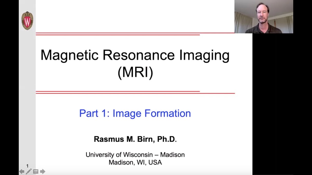
MRI Physics Fourier Transform for MRI Kucharczyk

Summary

This lecture focuses on MRI data processing and display, supplementing a previous talk on MRI physics. It explains how the Fourier transform is used to analyze the complex waveforms received by the MRI receiver coil, breaking them down into simpler sine waves of distinct frequencies and amplitudes. The presentation visually demonstrates how these waveforms can be represented in both the temporal and spatial domains, ultimately simplifying the data into a two-dimensional or three-dimensional k-space. This method allows for a comprehensive display of the MRI data, enabling a detailed understanding of the object scanned.

Takeaways

• 🧠 This talk serves as a supplement to a lecture on MRI physics, focusing on the processing and display of MRI data.
• 🔄 The Fourier transform is the primary mathematical tool used for processing MRI data, which involves complex waveforms of multiple frequencies and amplitudes.
• 📡 The MR receiver coil is responsible for receiving signals from the object being scanned, which are then processed.
• 🌊 The raw data from the coil is a complicated waveform that can be simplified using the Fourier transform into discrete frequencies and amplitudes.
• 📊 The presentation uses a simplified pictorial demonstration to explain how the Fourier transform processes and displays MRI data.
• 🌀 By adding waves of different frequencies and amplitudes, a complex waveform is created, which can be decomposed into simpler components using the Fourier transform.
• 📈 The data can be displayed in various ways, including as an amplitude versus frequency graph, making it easier to understand the composition of the waveform.
• 🔵 The amplitude and frequency of the signal can be represented as dots on a graph, which simplifies the visualization of complex data.
• 📐 The concept of the Fourier transform can be applied to both temporal (time-based) and spatial (distance-based) domains.
• 📊 The final display of MRI data is often in the form of a graph where each dot represents a frequency and amplitude at a specific spatial frequency, known as k-space.
• 🔗 The Fourier transform allows for the transformation of complex data into a sum of simple sine waves, which is essential for understanding the data obtained from MRI scans.

Q & A

What is the main purpose of the supplement to the lecture on MRI physics?

The supplement is created to address recurrent questions that have come up during the original lecture, providing a more detailed discussion and a recorded video for individual use at their convenience.

What is the role of the MR receiver coil in the MRI system?

The MR receiver coil is responsible for receiving the signal from the object being scanned. It captures an induced voltage consisting of multiple frequencies and amplitudes.

What mathematical tool is commonly used to process the raw data received by the MR receiver coil?

The Fourier transform is the mathematical tool most commonly used for processing the raw data received by the MR receiver coil.

How does the Fourier transform help in processing MRI data?

The Fourier transform allows for the decomposition of a complicated waveform, which consists of multiple frequencies and different amplitudes, into a sum of simple sine waves of discrete frequencies.

What is the significance of the amplitude and frequency in the context of MRI data?

In MRI data, the amplitude represents the strength of the signal at a particular frequency, while the frequency indicates the number of times a signal repeats over a period of time or distance.

How is the complex waveform resulting from the addition of multiple sine waves typically displayed?

The complex waveform resulting from the addition of multiple sine waves can be displayed as an amplitude versus frequency graph, where amplitude is represented by the height of blue columns on the frequency axis.

What is the difference between the temporal domain and the spatial domain in MRI data?

The temporal domain refers to variations over a unit of time, while the spatial domain refers to variations over a unit of distance. The Fourier transform can be applied to both domains to analyze the data.

How is spatial information that varies in two dimensions represented in MRI data?

Spatial information that varies in two dimensions is represented by considering both the x and y directions, with each having a specific frequency and amplitude, which can be displayed as dots in a two-dimensional Fourier space or k-space.

What is the term used for the pictorial representation of numerical values of frequencies and their amplitudes obtained from the MRI scanner?

The pictorial representation of numerical values of frequencies and their amplitudes obtained from the MRI scanner is referred to as two-dimensional Fourier space or simply two-dimensional k-space.

How can the Fourier transform be extrapolated to three dimensions in MRI data?

The Fourier transform can be extrapolated to three dimensions by collecting frequency data in the z direction, resulting in 3D Fourier space or 3D k-space, with the third dimension represented by kz in addition to kx and ky.

What is the typical representation of MRI data after applying the Fourier transform?

The typical representation of MRI data after applying the Fourier transform is a graph where the intensity of each dot represents the amplitude of each spatial frequency at a particular point, and the position of each dot represents the spatial frequency in each direction.

Outlines

00:00

🧠 MRI Data Processing and Display

This paragraph introduces the purpose of the video script, which is to supplement a lecture on MRI physics by addressing recurrent questions in greater detail. It explains the role of the MRI receiver coil in capturing signals from the object being scanned. The raw data received is a complex waveform consisting of multiple frequencies and amplitudes. The Fourier Transform is highlighted as the key mathematical tool used in MRI imaging to process this information. The script uses a simplified pictorial demonstration to explain how the Fourier Transform is applied to process and display MRI data. It starts with a basic sine wave example, showing how different waves with varying frequencies and amplitudes can be combined to form a complex waveform. The Fourier Transform allows this complex waveform to be decomposed into its constituent frequencies and amplitudes, which can be more easily analyzed and understood.

05:00

🌐 Fourier Transform in Spatial Domain

This paragraph delves into the application of the Fourier Transform in the spatial domain, contrasting it with the temporal domain. It uses an example of a line varying in whiteness over a unit of distance to illustrate how the Fourier Transform can be applied to analyze variations in functions over distance. The concept of frequency and amplitude is extended to the spatial domain, where the line's color variation is represented as a wave with a specific frequency and amplitude. The Fourier Transform is then used to simplify this data into a dot plot, where the position of the dot represents the frequency, and its brightness represents the amplitude. This method is extended to two-dimensional data, where variations in both the x and y directions are considered, leading to a more complex dot plot that represents the spatial frequencies and their amplitudes in both dimensions.

10:02

📊 Understanding MRI Data through K-Space

The final paragraph summarizes the concepts discussed in the script, focusing on the importance of frequency and the Fourier Transform in analyzing MRI data. It explains how the induced voltage in an MRI receiver coil is a complex waveform that can be decomposed into simple sine waves of discrete frequencies using the Fourier Transform. The conventional display of MRI data is described as a graph where the intensity of each dot represents the amplitude of each spatial frequency at a particular point in time, and the position of each dot represents the spatial frequency in each direction. The script introduces the concept of two-dimensional Fourier space or k-space, which is a pictorial representation of the numerical values of frequencies and their amplitudes obtained from the MRI scanner. The idea is extended to three dimensions, creating 3D Fourier space or 3D k-space. The paragraph concludes by emphasizing that a single graph can accurately display all the data obtained from every position in the object being scanned over the entire measurement time, providing a comprehensive view of the MRI data.

Keywords

💡MRI

Magnetic Resonance Imaging (MRI) is a non-invasive medical imaging technique used to visualize internal structures of the body in detail. In the context of the video, MRI is the primary subject, with a focus on how MRI data is processed and displayed. The video discusses the basics of MRI physics and the technology's ability to capture detailed images of the body's internal structures.

💡Fourier Transform

The Fourier Transform is a mathematical algorithm that decomposes complex signals into their frequency components. It is central to the video's discussion on MRI data processing, as it is used to analyze the waveforms received from the MRI scanner. The video explains how this tool simplifies the complex waveforms into discrete frequencies and amplitudes, which are then used to construct images.

💡Receiver Coil

The receiver coil is a component of the MRI system that captures the signal emitted by the object being scanned. The video emphasizes the role of the receiver coil in generating the initial data that is later processed using the Fourier Transform. It is the starting point for the data that will eventually be transformed into an MRI image.

💡Frequency

Frequency, in the context of the video, refers to the number of cycles per unit of time or space in a waveform. It is a key parameter in MRI data processing, as different frequencies correspond to different spatial features in the scanned object. The video uses frequency to explain how the Fourier Transform breaks down the complex waveforms into simpler components that can be visualized.

💡Amplitude

Amplitude is the measure of the magnitude or strength of a wave. In the video, amplitude is used to describe the strength of the signal received by the MRI receiver coil at different frequencies. It is a crucial factor in determining the intensity of the image produced, with higher amplitudes typically corresponding to brighter areas in the MRI image.

💡Waveform

A waveform is a graphical representation of a wave's amplitude over time. The video discusses how the raw data received by the MRI system is initially in the form of a complex waveform. This waveform is then processed using the Fourier Transform to extract the individual frequencies and amplitudes that contribute to the final image.

💡Spatial Domain

The spatial domain refers to the representation of a signal as it varies over space rather than time. The video explains that while the Fourier Transform is typically used for temporal data, it can also be applied to spatial data in MRI. This allows for the analysis of how the signal intensity varies across different points in space within the scanned object.

💡Temporal Domain

The temporal domain is the representation of a signal as it varies over time. In the video, the temporal domain is contrasted with the spatial domain to illustrate how the Fourier Transform can be applied to both. The initial complex waveforms received by the MRI system are analyzed in the temporal domain before being transformed into spatial data for imaging.

💡k-space

k-space, or Fourier space, is a conceptual space used in MRI to represent the spatial frequencies of the image. The video describes how the Fourier Transform is used to map the data from the receiver coil into k-space, where each point represents a different spatial frequency and amplitude. This mapping is essential for reconstructing the final MRI image.

💡Sine Wave

A sine wave is a continuous wave that oscillates sinusoidally. The video uses sine waves as an example to illustrate how simple waveforms with specific frequencies and amplitudes can be combined to form more complex waveforms. This concept is foundational to understanding how the Fourier Transform decomposes complex MRI data into its constituent frequencies and amplitudes.

Highlights

The talk supplements a lecture on MRI physics, focusing on processing and display of MRI data.

The MR receiver coil receives signals from the object being scanned, inducing a complex voltage waveform.

The Fourier transform is the primary mathematical tool for processing MRI data, used for almost all MR imaging.

A simplified pictorial demonstration of the Fourier transform is presented to explain its role in MRI data processing.

The waveform's frequency and amplitude are key parameters described in the talk.

Adding waves of different frequencies and amplitudes results in a complex waveform.

The Fourier transform allows for the decomposition of a complex waveform into its constituent frequencies and amplitudes.

Data can be displayed as an amplitude versus frequency graph, simplifying the interpretation of complex waveforms.

The relationship between a complex waveform and its frequency components is illustrated through the Fourier transform.

The Fourier transform is also applicable to the spatial domain, analyzing variations over distance.

A line varying in whiteness over a unit of distance is used to demonstrate the spatial domain analysis.

The concept of frequency in the spatial domain is introduced, with the line having a frequency of one cycle per meter.

The Fourier transform can be applied to two-dimensional data, such as variations in both the x and y directions.

The talk explains how to represent two-dimensional spatial information using a combination of frequencies and amplitudes.

The concept of two-dimensional Fourier space or k-space is introduced to represent spatial frequencies.

The extension of the Fourier transform to three dimensions is discussed, creating 3D Fourier space or 3D k-space.

Frequency is defined as the number of repetitions over a period of time or distance.

The Fourier transform decomposes a complicated waveform into simple sine waves of discrete frequencies.

MRI data is typically displayed as a graph where the intensity of each dot represents the amplitude of a spatial frequency.

The position of each dot in the graph represents the spatial frequency in each direction.

A single graph can show all data obtained from every position in the object being scanned over the entire measurement time.

The typical representation of MRI data is a single picture, summarizing the entire scan's data.

Transcripts

this talk is on the processing

and display of mri data it is intended

to be a supplement

to a lecture that i have frequently

given with professor don plewis

on the basics of mri physics which we

call spin gymnastics

this supplement is created because of

questions that that have come to us on a

recurrent basis

on certain parts of the original

talk therefore

we felt it would be worthwhile to go

over

certain of these questions in greater

detail

and then to record the talk

as a video and have it available for

each individual's use

at the individual's convenience

this short presentation

will discuss how mri data

is processed and displayed

the mr receiver coil is the part of the

mri system

that receives signal from the object

being scanned

the data that is received by the coil is

an induced voltage in the coil

consisting of multiple frequencies

and amplitudes it has a very complicated

waveform in its raw state

the fourier transform is the

mathematical tool most commonly used for

processing this type

of information and is used for almost

all

mr imaging this presentation is a

simplified pictorial demonstration of

the fourier transform

and how the fourier transform is used to

process

and display mri data

let's look at a wave as it evolves

over time we'll start with something

very simple

we look at this sine wave it goes

through one

full cycle over one second

and we have assigned an arbitrary scale

to the vertical axis

we see it has an amplitude of

three units above the baseline so we

would describe

this wave as having a frequency of one

cycle per second an

amplitude of three units which we could

represent

in textual form as we see in the upper

left

or simply as a pair of numbers a one

in a three let's look at a couple

other waves of different frequencies and

different amplitudes

the next one has a frequency of three

cycles

over one second and it has an amplitude

of one

the next wave has a frequency of eight

cycles per second

and an amplitude of two units

if we then add all these waves together

over each fraction of a second

we would display it as the graph

on the bottom it looks like a pretty

complicated waveform

it would be difficult to tell what the

component frequencies and the component

amplitudes are of the frequencies that

contribute to this wave

because the this wave is composed of

multiple different frequencies in the

amplitude varies

another way of displaying the the same

data

is as follows if we look

in the upper row that same

data could be displayed as an amplitude

versus frequency graph where the

amplitude is displayed as a blue column

of three units tall

and placed on the frequency axis that

represents

one cycle per second similarly we could

do this

with the other graphs

as shown in the next row down

this is a frequency of three with an

amplitude

of one unit the next one

uh demonstrates that the frequency

is eight cycles per second and has an

amplitude

of two units and if we now add all

this data together it's a much simpler

way of

looking at the data we see that it's

composed of three discrete

frequencies each of different amplitudes

so if we're going the reverse direction

using

the waveforms in the leftmost column it

would be difficult to

disassemble the complicated waveform

into its individual components

amplitudes but if we look at the middle

column

it's a relatively simple task the

relationship between the leftmost column

and the middle column is the fourier

transform

and then we can take this one step

further

and if we look at the bottom row rather

than

displaying the amplitudes

as the height of blue columns

we could simply represent them as dots

on a single linear axis where the

either the size or the brightness of the

dot represents the amplitude at the

particular frequency

remembering of course that these graphs

are a pictorial representation of

certain numbers

so if we take a second look at the

bottom right

we see that that complicated waveform

consists

of frequencies of one cycle per second

with an amplitude of three

three cycles per second with an

amplitude of one

and eight cycles per second of

amplitude 2.

the same type of analysis

can be carried out for things

or functions that vary over a unit of

distance

rather than over a unit of time and this

is called the spatial domain

rather than the temporal domain

so in this example i have drawn

a relatively thick line across the

top left of the image that

varies in whiteness going from left to

right

it starts as a neutral gray it becomes

white then becomes gray then becomes

black

and becomes gray again so it's gone over

one full cycle in color variation over

a unit of distance of one meter

so in the spatial domain it would be

said that this line has a frequency of

one cycle per meter

and if we assigned numbers to the gray

scale

where gray is zero and white is three

we would say that the white part

of this line has an amplitude of three

above the baseline grayscale

and we could represent it as a wave

over a distance of one meter where the

amplitude of the wave varies from zero

representing gray

up to three representing white back to

zero representing gray

minus three representing black and back

to zero

representing gray

if we then did the same type of fourier

transform

on this line we could represent it the

same way

we could represent it as having an

amplitude of 3 units

in this case units of whiteness at a

frequency

of one cycle over a meter

and then we could collapse this data

down further

into a dot if we wish to so display the

information

as a single dot on the frequency

axis at the position of one cycle per

meter

and the brightness of the dot would have

an amplitude of three

so this works very well for something

that varies

in one dimension how about if it varies

in two dimensions

well if we try to represent that data

in the bottom left hand image that

square

that single white dot of amplitude 3

would only represent

the function

the variation in signal intensity

in the x direction and if it has no

variation in the white in the y

direction it would be adequate

but what if something also varied in the

y direction

let's look at the situation

if we have spatial information

that varies in two directions

on the bottom we have the example we

have previously seen

where we have spatial information that

varies over one

cycle per meter in the x direction and

we've represented it

as a single white dot of amplitude three

on the x frequency direction

equal to one cycle per meter

if we now have a second

a square where the variation

in signal intensity is in the vertical

or y direction

and we change the frequency to

three cycles of variation over

one meter of distance in that vertical

or y direction

we'd have we would say it has three

cycles per meter

in the y direction and we've changed the

amplitude

to have an amplitude of 2 rather than

amplitude of 3.

if we put these two things together we

would get an image like that

but we could decompose that and

represent it as a frequency

in the x direction as already shown of

one with amplitude three and a frequency

in the y direction of

frequency 3 and amplitude 2.

if we did this for every possible

frequency

say up to 128 or 256 different

frequencies

each of different amplitudes we would

end up displaying

these dots in

the x and y directions and it would look

like this

and what this is is a pictorial

representation

of amplitudes which is represented by

the intensity of each point

of each spatial frequency in each of the

x

in y directions which is determined by

the position of the point

the axes when we're dealing with spatial

frequencies

are conventionally labeled as k sub x

and k sub y but

it's important not to lose

site of the fact that each dot in this

single graph represents

a frequency in the x direction a

frequency in the right direction

and an amplitude of those frequencies

so what we saw at the last part of the

last slide

was this picture this is a pictorial

representation

of the numerical values of the

frequencies and their amplitudes that

come out of the mri scanner into the mri

receiver coil and it is

referred to as t two dimensional fourier

space

or simply as two-dimensional k space

uh the same

uh can be extrapolated to three

dimensions if you collect data

a frequency data in the z direction so

the third dimension becomes

kz in addition to kx and ky

and in this case we have 3d fourier

space

or 3d k space

this brings us to the summary frequency

is the number of times that something is

repeated over a period of time

or over a distance in space

the fourier transform is a mathematical

tool that allows a complicated waveform

consisting of multiple frequencies and

different amplitudes

to be decomposed into a sum of simple

sine waves of discrete frequencies

the induced voltage in an mri receiver

is this type of complicated waveform

so it lends itself well for fourier

analysis the conventional way of

displaying this mri data is a graph

where the intensity of each dot

represents the amplitude

of each spatial frequency at a

particular point in time

the position of each dot represents the

spatial frequency

in each direction and units of cycles

per unit length

to conclude a single graph can

accurately

show all the data obtained from every

position

in the object being scanned over the

entire measurement time

it can be displayed as a single picture

and the typical representation

is shown at the bottom right

that brings us to the end of this short

lecture thank you for your attention