Time Series Talk : Autoregressive Model

Summary

This video delves into the Autoregressive (AR) model, a favored method for time series forecasting. It emphasizes the model's strength in predicting future values based on past data, using a milk distributor's monthly demand as an example. The presenter introduces the concept of auto regression, discusses the importance of selecting relevant lags to avoid overfitting, and employs the Partial Autocorrelation Function (PACF) chart to determine the optimal model. The simplicity and intuitive nature of AR models are highlighted, making them accessible for viewers new to time series analysis.

Takeaways

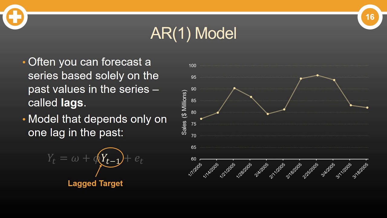
• 📈 The script introduces the AR (Auto-Regressive) model, a time series forecasting model that predicts future values based on past values of the same variable.
• 🔍 The importance of using past values for prediction is emphasized, as it's a natural approach to forecasting, considering the inherent patterns in time series data.
• 🚚 The example of a milk distributor needing to predict monthly milk demand illustrates the practical application of the AR model in a business context.
• 📊 A visual representation of milk demand over time is suggested, highlighting the cyclical pattern that can be leveraged for prediction.
• 📝 The notation M_t for current month's demand and M_t-1, M_t-2, etc., for past demands is introduced to formalize the model.
• ❌ The script warns against overfitting by including too many lags in the model, advocating for a simpler model that captures the essential patterns.
• 📉 The concept of partial autocorrelation function (PA CF) is introduced as a tool to determine which lags have a significant direct effect on the current demand.
• 📈 The PA CF chart helps in selecting relevant lags for the model by identifying those with significant correlations outside the confidence bands.
• 📝 A potential AR model is outlined, including an intercept, coefficients for selected lags, and an error term, based on the PA CF analysis.
• 🔧 The script suggests that the chosen model should be tested and refined, acknowledging that while the basics are covered, further complexities will be discussed in future videos.
• 👍 The presenter expresses a preference for the AR model due to its simplicity and intuitive approach to forecasting based on past values.

Q & A

What is the main topic of the video?

The main topic of the video is time series forecasting, specifically focusing on the Autoregressive (AR) model.

What does 'autoregressive' mean in the context of the AR model?

In the context of the AR model, 'autoregressive' means that the model predicts future values of a variable based on its own past values.

Why is the AR model considered powerful in time series forecasting?

The AR model is considered powerful because it leverages the natural pattern of a variable's past values to predict its future values, which can lead to stronger predictions if a pattern emerges.

What is the example scenario used in the video to illustrate the AR model?

The example scenario is that of a milk distributor who wants to predict the monthly demand for milk to avoid overproduction or undersupply.

What is the significance of plotting the quantity of milk demanded over time?

Plotting the quantity of milk demanded over time helps to visualize patterns and trends that can be used to make predictions about future demand.

What notation is introduced to represent the quantity of milk demanded in the video?

The notation introduced is M sub T for the quantity of milk demanded in the current month, and M sub t minus n for the quantity demanded n months ago.

Why might including all lags from 1 through 12 in the model be problematic?

Including all lags from 1 through 12 might lead to overfitting, where the model is too closely tuned to the specific data and may not generalize well over time.

What is the role of the partial autocorrelation function (PACF) in selecting lags for the AR model?

The PACF helps in determining which lags have a significant direct correlation with the current period's milk demand, excluding the effects of intermediate periods, thus guiding the selection of important lags for the model.

How does the video suggest determining the best AR model for the milk demand forecasting scenario?

The video suggests using the PACF plot to identify lags with significant direct correlations and then constructing an AR model that includes those lags.

What is the importance of preferring a simpler model when possible in regression modeling?

A simpler model is preferred when it can perform as well as a more complex model because it is likely to be more robust and hold up better over time, avoiding issues like overfitting.

What does the video suggest as the next steps after constructing the AR model?

The video suggests that after constructing the AR model based on the PACF plot, the next steps would involve testing the model and considering other factors that might influence milk demand in future videos.