Describing Distributions: Center, Spread & Shape | Statistics Tutorial | MarinStatsLectures
Summary
TLDRThis script discusses the verbal description of the shape, center, and spread of a numeric variable's distribution. It introduces the concept of symmetry and skewness in distributions, using examples to illustrate symmetric, skewed right, and skewed left distributions. The script also touches on the importance of anticipating distribution shapes for variables like income, height, and class grades before data collection. It sets the stage for future discussions on more quantitative measures of distribution, such as mean, median, standard deviation, and interquartile range.
Takeaways
- 📊 Describing a numeric variable's distribution involves discussing its shape, center, and spread.
- 🔍 Histograms and box plots are useful for summarizing the distribution of numeric variables visually.
- 📈 The shape of a distribution can be symmetric or skewed, with skewness being towards the right (positive) or left (negative).
- 📚 A normal distribution is symmetric and bell-shaped, often used as a reference for many natural phenomena.
- 🤔 When considering the distribution of variables like income, height, or grades, it's helpful to predict their shape before data collection.
- 💼 Income distributions are often skewed right due to a lower bound and a long tail towards higher values.
- 🚹 Adult height distributions tend to be more symmetric and bell-shaped, with people evenly distributed around the average height.
- 📚 Grade distributions are typically skewed left or negatively skewed because they are capped at 100 and often have a lower tail towards zero.
- 📐 Measures of location, such as mean, median, and quartiles, help pinpoint the center of a distribution.
- 📉 Measures of spread or variability, like standard deviation, variance, and interquartile range, quantify how spread out the data is.
- 🔢 Quantitative descriptions of center and spread will be explored in more detail in subsequent videos, moving beyond qualitative descriptors.
Q & A
What are the two main characteristics of a distribution that are verbally described?
-The two main characteristics of a distribution that are verbally described are the shape of the distribution and the center and spread of the data.
What does a symmetric distribution imply about the data?
-A symmetric distribution implies that the data is evenly distributed around the center point, with both sides mirroring each other.
What is the term used to describe a distribution that is not symmetric and tails out to one side?
-A distribution that is not symmetric and tails out to one side is described as 'skewed.'
How is a distribution that tails out towards the right side characterized?
-A distribution that tails out towards the right side is characterized as 'positively skewed' or 'skewed right.'
What is meant by a 'normal' or 'bell-shaped' distribution?
-A 'normal' or 'bell-shaped' distribution refers to a symmetric distribution that decreases evenly on either side of the center, resembling the shape of a bell.
What is the expected shape of the distribution for individual incomes?
-The expected shape of the distribution for individual incomes is often 'skewed right,' indicating a lower bound with few individuals at the higher end.
Why are adult heights often symmetrically distributed?
-Adult heights are often symmetrically distributed because there is an average height, and people are evenly distributed above and below this average.
What is the typical distribution shape for class grades, and why?
-Class grades typically have a 'negatively skewed' or 'skewed left' distribution because grades are bounded between 0 and 100, with many students scoring above 50 and fewer scoring very low or very high.
What are some measures of location that can be verbally described for a distribution?
-Measures of location that can be verbally described for a distribution include the mean, median, maximum, minimum, and quartiles.
How is the spread or variability of a distribution verbally described?
-The spread or variability of a distribution is verbally described by terms like 'spread out,' 'variable,' 'tight,' or 'concentrated,' based on how the data points are dispersed around the center.
What are some quantitative measures that will be used to describe the center and spread of a distribution in future videos?
-Some quantitative measures that will be used to describe the center and spread of a distribution include mean, median, standard deviation, variance, and interquartile range.
Outlines

此内容仅限付费用户访问。 请升级后访问。
立即升级Mindmap

此内容仅限付费用户访问。 请升级后访问。
立即升级Keywords

此内容仅限付费用户访问。 请升级后访问。
立即升级Highlights

此内容仅限付费用户访问。 请升级后访问。
立即升级Transcripts

此内容仅限付费用户访问。 请升级后访问。
立即升级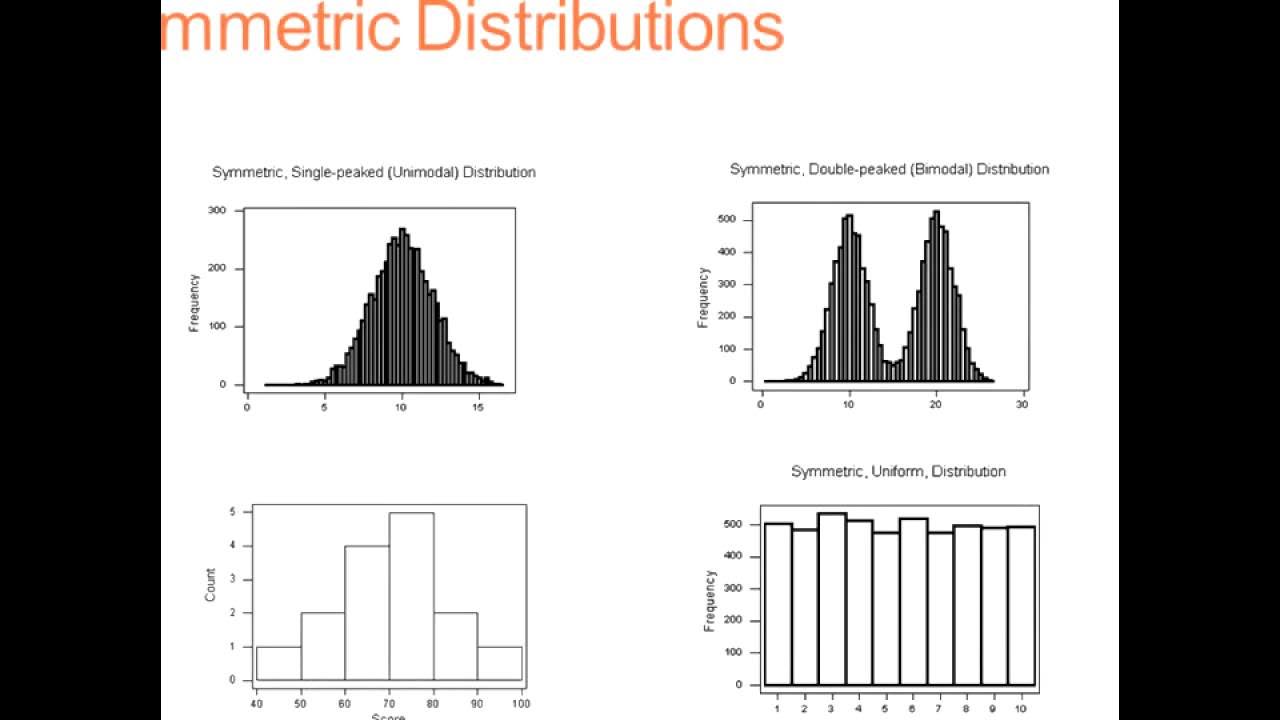


5.0 / 5 (0 votes)
