The Essential Main Ideas of Neural Networks

Summary

This video explains neural networks, which identify patterns in data to make predictions, using the analogy of fitting a 'green squiggle' to a dataset. It introduces core neural network concepts like nodes, connections, hidden layers, and activation functions. Though neural networks seem complicated, they are essentially 'big fancy squiggle fitting machines' that use basic math operations on bent lines to generate new shapes. By adding and manipulating these shapes, neural networks can model incredibly complex datasets for machine learning tasks. This friendly beginner's guide aims to demystify neural networks by breaking things down step-by-step.

Takeaways

• 😀 Neural networks fit squiggles to data to make predictions
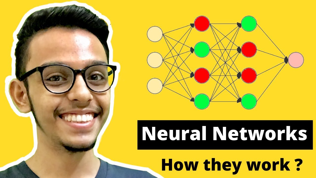
• 👉 Nodes are connected in layers to transform activation functions into new shapes
• 📈 Weights and biases parameterize connections to reshape activation functions
• 🔍 Looking inside the neural network black box demystifies how they work
• 📊 Backpropagation estimates optimal parameters by fitting the network to data
• ⚙️ More layers and nodes enable more complex squiggle fitting for tricky data
• 🧠 Neural networks were named by analogy to biological neurons and synapses
• ✏️ Simple math and labeled diagrams provide intuition into neural mechanisms
• 🎓 This tutorial series aims to develop deep understanding of neural networks
• 🚀 Even simple networks demonstrate the power and flexibility of the approach

Q & A

What is the goal of the StatQuest video series on neural networks?

The goal is to take a peek inside the neural network 'black box' by breaking down each concept and technique into its components and walking through how they fit together step-by-step.

What type of activation function is used in the example neural network?

The soft plus activation function is used in the example neural network.

Why are the layers between the input and output nodes called hidden layers?

The layers between the input and output nodes are called hidden layers because their values are not directly observed in the training data.

What are the two key components that allow a neural network to create new shapes?

The two key components are the activation functions, which create bent or curved lines, and the weights and biases on the connections, which reshape and combine these lines.

What is backpropagation and when will it be discussed?

Backpropagation is the method used to estimate the parameters (weights and biases) when fitting a neural network to data. It will be discussed in Part 2 of the video series.

Why are neural networks called 'big fancy squiggle fitting machines'?

Because their key functionality is using activation functions and weighted connections to fit complicated squiggly lines (green squiggles) to data.

What math notation is used for the log function in the video?

The natural log, or log base e, is used in the math notation.

How many nodes are in the hidden layer of the example neural network?

There are 2 nodes in the single hidden layer of the example neural network.

What are some ways you can support the StatQuest channel and quest on?

Ways to support include subscribing, contributing to Josh's Patreon campaign, becoming a channel member, buying songs/merchandise, or donating.

Why are neural networks still called neural networks if nodes aren't really like neurons?

They were originally inspired by and named after neurons and synapses back when they were first invented in the 1940s/50s, even if the analogy isn't perfect.

Outlines

00:00

😊 Introducing Neural Networks

The narrator Josh introduces neural networks, stating they seem complicated but can be broken down into understandable components. He outlines the goals for this video series on neural networks, which includes labeling all parts of a simple neural network to show how it fits a curve to data through basic math.

05:02

🧠 Understanding Activation Functions

The narrator defines the curved lines inside nodes of a neural network as activation functions. Common options include sigmoid, ReLU (rectified linear unit), and soft plus. The choice impacts the shape the neural network can fit. This example uses soft plus.

10:05

📈 Fitting Curves with Neural Networks

The narrator steps through the math to show how a simple neural network with one input node and two hidden nodes can fit a curve to data. Each hidden node slices and scales its activation function differently based on the weights and biases estimated when fitting the network.

15:06

✅ Making Predictions from the Fitted Curve

The narrator combines the curves from the two hidden nodes into a final fitted curve that matches the data. He shows how new data can be input to generate a prediction from the corresponding point on the final fitted curve. Finally, he explains the biological inspiration for neural networks.

Keywords

💡Neural network

A neural network is a type of machine learning algorithm that is designed to recognize patterns in data. It consists of an input layer, one or more hidden layers, and an output layer, with nodes in each layer and connections between the nodes. In the video, neural networks are used to fit a squiggle (nonlinear function) to the drug dosage data to predict treatment effectiveness.

💡Activation function

The activation function is a curved or bent line inside each node of the neural network. It transforms the input from the previous layer nonlinearly before passing it to the next layer. Common activation functions mentioned are sigmoid, ReLU (rectified linear unit), and soft plus. The video uses soft plus activation functions to reshape the data.

💡Backpropagation

Backpropagation is an algorithm used to train neural networks. It estimates the parameters (weights and biases) for the connections in the network by comparing its predictions on the training data to the actual targets, calculating the error, and adjusting the parameters to reduce the error. The estimated parameters result in different transformations of the activation function curves.

💡Hidden layer

The hidden layers are the intermediate layers of nodes between the input and output layers in a neural network. They enable the model to learn more complex nonlinear relationships between inputs and outputs. Deciding how many hidden layers and how many nodes in each layer is important for good performance.

💡Weight

The weights are parameter values that are multiplied with the input values as they pass from one node to the next. They determine how much influence the input to a node has on the output. The backpropagation algorithm adjusts the weights during training to minimize error.

💡Bias

The biases are parameter values that are added to the weighted input in nodes of the neural network after multiplication by the weights. Together with the weights, they control the transformation applied to activation functions.

💡Overfitting

Overfitting refers to a model that fits the training data very well but fails to generalize to new data. The video explains that neural networks can fit arbitrarily complex squiggles to data, avoiding overfitting is important. Techniques like regularization and dropout help prevent overfitting.

💡Generalization

Generalization refers to how well a machine learning model can adapt what is learned from the training data to make accurate predictions on new unseen data. The video talks about neural networks being universal approximators that can fit to almost any dataset, enabling good generalization.

💡Nonlinearity

Most real-world data has nonlinear relationships that cannot be modeled with linear functions. Neural networks introduce nonlinearity through the activation functions, allowing them to fit nonlinear squiggles to data and model complex nonlinear patterns.

💡Universal approximation

This refers to the ability of neural networks with at least one hidden layer to represent a wide range of nonlinear functions, making them universal approximators. This theoretical capability enables them to model complex real-world data.

Highlights

Neural networks cover a broad range of concepts and techniques, however, people call them a black box because it can be hard to understand what they're doing.

The goal of this series is to take a peek into the black box by breaking down each concept and technique into its components and walking through how they fit together, step by step.

In this first part, we will learn about what neural networks do, and how they do it.

I have a new way to think about neural networks that will help beginners and seasoned experts alike gain a deep insight into what neural networks do.

The math will be as simple as possible, while still being true to the algorithm. These differences will help you develop a deep understanding of what neural networks actually do.

We're going to use this super simple dataset and show how this neural network creates this green squiggle.

The curved or bent lines are called activation functions. When you build a neural network you have to decide which activation function, or functions, you want to use.

Although there are rules of thumb for making decisions about the hidden layers, you essentially make a guess and see how well the neural network performs, adding more layers and nodes if needed.

In theory, neural networks can fit a green squiggle to just about any dataset, no matter how complicated, and i think that's pretty cool.

If you want to review statistics and machine learning offline check out the StatQuest study guides at statquest.org. There's something for everyone.

If you like this StatQuest and want to see more, please subscribe.

And if you want to support StatQuest consider contributing to my patreon campaign, becoming a channel member, buying one or two of my original songs, or a t-shirt, or a hoodie, or just donate.

This neural network starts with two identical activation functions, but the weights and biases on the connections slice them, flip them, and stretch them into new shapes, which are then added together to get a squiggle that is entirely new.

Just imagine what types of green squiggles we could fit with more hidden layers and more nodes in each hidden layer.

I think neural networks should be called big fancy squiggle fitting machines, because that's what they do.

Transcripts

Neural networks...

seem so complicated, but they're not!

StatQuest!

Hello!

I'm Josh Starmer and welcome to StatQuest!

Today, we're going to talk about neural networks, part one: inside the black box!

Neural networks, one of the most popular algorithms in machine learning, cover a broad range of concepts and techniques.

however, people call them a black box because it can be hard to understand what they're doing.

the goal of this series is to take a peek into the black box by breaking down each

concept and technique into its components and walking through how they fit together, step by step.

in this first part, we will learn about what neural networks do, and how they do it.

in part two, we'll talk about how neural networks are fit to data with backpropagation.

then, we will talk about variations on the simple neural network presented in this part, including deep learning.

note: crazy awesome news!

i have a new way to think about neural networks that will help beginners and seasoned

experts alike gain a deep insight into what neural networks do.

for example, most tutorials use cool looking, but hard to understand graphs, and fancy

mathematical notation to represent neural networks.

in contrast, i'm going to label every little thing on the neural network to make it easy to keep track of the details.

and the math will be as simple as possible, while still being true to the algorithm.

these differences will help you develop a deep understanding of what neural networks actually do.

so, with that said, let's imagine we tested a drug that was designed to treat an illness

and we gave the drug to three different groups of people, with three different dosages: low, medium, and high.

the low dosages were not effective so we set them to zero on this graph. in contrast,

the medium dosages were effective so we set them to one.

and the high dosages were not effective, so those are set to zero.

now that we have this data, we would like to use it to predict whether or not a future dosage will be effective.

however we can't just fit a straight line to the data to make predictions, because

no matter how we rotate the straight line, it can only accurately predict two of the three dosages.

the good news is that a neural network can fit a squiggle to the data.

the green squiggle is close to zero for low dosages, close to one for medium dosages,

and close to zero for high dosages. and even if we have a really complicated dataset

like this, a neural network can fit a squiggle to it.

in this StatQuest we're going to use this super simple dataset and show how this neural network creates this green squiggle.

but first, let's just talk about what a neural network is.

a neural network consists of nodes and connections between the nodes.

note: the numbers along each connection represent parameter values that were estimated

when this neural network was fit to the data.

for now, just know that these parameter estimates are analogous to the slope and intercept

values that we solve for when we fit a straight line to data.

likewise, a neural network starts out with unknown parameter values that are estimated

when we fit the neural network to a dataset using a method called backpropagation.

and we will talk about how backpropagation estimates these parameters in part 2 in this series.

but, for now, just assume that we've already fit this neural network to this specific

dataset, and that means we have already estimated these parameters.

also, you may have noticed that some of the nodes have curved lines inside of them.

these bent or curved lines are the building blocks for fitting a squiggle to data.

the goal of this StatQuest is to show you how these identical curves can be reshaped

by the parameter values and then added together to get a green squiggle that fits the data.

note: there are many common bent or curved lines that we can choose for a neural network.

this specific curved line is called soft plus, which sounds like a brand of toilet paper.

alternatively, we could use this bent line, called ReLU, which is short for rectified linear unit, and sounds like a robot.

or, we could use a sigmoid shape, or any other bent or curved line.

oh no!

it's the dreaded terminology alert!

the curved or bent lines are called activation functions.

when you build a neural network you have to decide which activation function, or functions, you want to use.

when most people teach neural networks they use the sigmoid activation function.

however, in practice, it is much more common to use the ReLU activation function, or the soft plus activation function.

so we'll use the soft plus activation function in this StatQuest.

anyway, we'll talk more about how you choose activation functions later in this series.

note: this specific neural network is about as simple as they get.

it only has one input node, where we plug in the dosage, only one output node to tell

us the predicted effectiveness, and only two nodes between the input and output nodes.

however, in practice, neural networks are usually much fancier and have more than

one input node, more than one output node, different layers of nodes between the

input and output nodes, and a spider web of connections between each layer of nodes.

oh no!

it's another terminology alert!

these layers of nodes between the input and output nodes are called hidden layers.

when you build a neural network one of the first things you do is decide how many

hidden layers you want and how many nodes go into each hidden layer.

although there are rules of thumb for making decisions about the hidden layers, you

essentially make a guess and see how well the neural network performs, adding more layers and nodes if needed.

now, even though this neural network looks fancy, it is still made from the same parts

used in this simple neural network, which has only one hidden layer with two nodes.

so let's learn how this neural network creates new shapes from the curved or bent

lines in the hidden layer, and then adds them together to get a green squiggle that fits the data.

note: to keep the math simple, let's assume dosages go from zero, for low, to one, for high.

the first thing we are going to do is plug the lowest dosage, zero, into the neural network.

now, to get from the input node to the top node in the hidden layer, this connection

multiplies the dosage by negative 34.4 and then adds 2.14, and the result is an x-axis coordinate for the activation function.

for example, the lowest dosage 0 is multiplied by negative 34.4, and then we add 2.14,

to get 2.14 as the x-axis coordinate for the activation function.

to get the corresponding y-axis value we plug 2.14 into the activation function, which in this case is the soft plus function.

note: if we had chosen the sigmoid curve for the activation function then we would

plug 2.14 into the equation for the sigmoid curve.

and if we had chosen the ReLU bent line for the activation function, then we would plug 2.14 into the ReLU equation.

but, since we are using soft plus for the activation function, we plug 2.14 into the soft plus equation.

and the log of one plus e raised to the 2.14 power is 2.25.

note: in statistics, machine learning, and most programming languages, the log function

implies the natural log, or the log base e. anyway, the y-axis coordinate for the

activation function is 2.25, so let's extend this y-axis up a little bit and put

a blue dot at 2.25 for when dosage equals zero.

now, if we increase the dosage a little bit and plug 0.1 into the input, the x-axis

coordinate for the activation function is negative 1.3, and the corresponding y-axis

value is 0.24. so, let's put a blue dot at 0.24 for when dosage equals 0.1. and,

if we continue to increase the dosage values all the way to 1, the maximum dosage, we get this blue curve.

note: before we move on I want to point out that the full range of dosage values,

from 0 to 1, corresponds to this relatively narrow range of values from the activation function.

in other words, when we plug dosage values, from 0 to 1, into the neural network,

and then multiply them by negative 34.4 and add 2.14, we only get x-axis coordinates that are within the red box.

and thus, only the corresponding y-axis values in the red box are used to make this new blue curve.

bam!

now we scale the y-axis values for the blue curve by negative 1.3. for example, when

dosage equals zero the current y-axis coordinate for the blue curve is 2.25, so we

multiply 2.25 by negative 1.3 and get negative 2.93. and negative 2.93 corresponds to this position on the y-axis.

likewise, we multiply all of the other y-axis coordinates on the blue curve by negative

1.3 and we end up with a new blue curve.

bam!

now, let's focus on the connection from the input node, to the bottom node in the hidden layer.

however, this time, we multiply the dosage by negative 2.52, instead of negative 34.4,

and we add 1.29, instead of 2.14, to get the x-axis coordinate for the activation function.

remember, these values come from fitting the neural network to the data with backpropagation,

and we'll talk about that in part two in this series.

now, if we plug the lowest dosage, zero, into the neural network, then the x-axis

coordinate for the activation function is 1.29.

now we plug 1.29 into the activation function to get the corresponding y-axis value,

and get 1.53. and that corresponds to this yellow dot.

now, we just plug in dosage values from 0 to 1 to get the corresponding y-axis values, and we get this orange curve.

note: just like before, i want to point out that the full range of dosage values,

from 0 to 1, corresponds to this narrow range of values from the activation function.

in other words, when we plug dosage values from 0 to 1 into the neural network we

only get x-axis coordinates that are within the red box.

and thus, only the corresponding y-axis values in the red box are used to make this new orange curve.

so we see that fitting a neural network to data gives us different parameter estimates

on the connections and that results in each node in the hidden layer using different

portions of the activation functions to create these new and exciting shapes.

now, just like before, we scale the y-axis coordinates on the orange curve, only this

time we scale by a positive number: 2.28.

beep boop beep! for every number written on the screen] and that gives us this new orange curve.

now the neural network tells us to add the y-axis coordinates from the blue curve

to the orange curve, and that gives us this green squiggle.

then, finally, we subtract 0.58 from the y-axis values on the green squiggle, and

we have a green squiggle that fits the data.

bam!

now, if someone comes along and says that they are using dosage equal to 0.5 we can

look at the corresponding y-axis coordinate on the green squiggle and see that the dosage will be effective.

or, we can solve for the y-axis coordinate by plugging dosage equals 0.5 into the neural network, and do the math.

[Music] and we see that the y-axis coordinate on the green squiggle is 1.03, and since

1.03 is closer to 1 than 0, we will conclude that a dosage equal to 0.5 is effective.

double bam!

now, if you've made it this far you may be wondering why this is called a neural network.

instead of a big fancy squiggle fitting machine.

the reason is that way back in the 1940s and 50s, when neural networks were invented,

they thought the nodes were vaguely like neurons, and the connections between the nodes were sort of like synapses.

however, i think they should be called big fancy squiggle fitting machines, because that's what they do.

note: whether or not you call it a squiggle fitting machine, the parameters that we

multiply are called weights, and the parameters that we add are called biases.

note: this neural network starts with two identical activation functions, but the

weights and biases on the connections slice them, flip them, and stretch them into

new shapes, which are then added together to get a squiggle that is entirely new.

and then the squiggle is shifted to fit the data.

now, if we can create this green squiggle with just two nodes in a single hidden layer,

just imagine what types of green squiggles we could fit with more hidden layers and more nodes in each hidden layer.

in theory, neural networks can fit a green squiggle to just about any dataset, no

matter how complicated, and i think that's pretty cool.

triple bam!

now it's time for some shameless self-promotion!

if you want to review statistics and machine learning offline check out the StatQuest study guides at statquest.org.

there's something for everyone.

hooray!

we've made it to the end of another exciting StatQuest.

if you like this StatQuest and want to see more, please subscribe.

and if you want to support StatQuest consider contributing to my patreon campaign,

becoming a channel member, buying one or two of my original songs, or a t-shirt, or a hoodie, or just donate.

the links are in the description below.

alright, until next time.

quest on!