Operations Research 06A: Transportation Problem
Summary
TLDRThis video script introduces the transportation problem, a special linear programming (LP) issue with practical applications, which can be solved more efficiently using specialized algorithms than the traditional simplex method. It outlines the problem setup involving supply and demand points, shipping costs, and capacity constraints. The script explains the formulation of both balanced and unbalanced transportation problems, the use of dummy nodes for balancing, and the advantages of the transportation simplex method over the regular simplex method for solving these problems.
Takeaways
- 📚 The video discusses the formulation of transportation problems, a special type of Linear Programming (LP) problem with practical applications.
- 🔍 While the simplex method can solve transportation problems, specialized algorithms are more efficient due to the unique structure of these problems.
- 📦 The goal of a transportation problem is to determine the best way to meet the demand of multiple customers using the supply from various sources, considering shipping costs.
- 🏭 An example given involves two factories supplying three customers, with unit shipping costs varying based on distance and factory capacity limits.
- 🔢 Decision variables x_{ij} represent the number of products shipped from one factory to a customer, and the objective function calculates the total shipping cost.
- 🚫 Constraints ensure that each factory does not exceed its capacity and each customer's demand is met.
- 📉 The script introduces the concept of a balanced transportation problem, where total supply equals total demand, contrasting with the general case.
- 🔄 For balanced problems, the transportation simplex method is an efficient algorithm, which will be covered in a different video.
- 📈 The transportation tableau is a visual representation of the problem, showing supply and demand nodes, shipping costs, and decision variables.
- 🔄 Unbalanced problems require the introduction of dummy supply or demand nodes to balance the total supply with the total demand, using penalties for unmet demand.
- 🛠 The transportation simplex method is preferred over the regular simplex method for balanced problems due to its ability to handle equality constraints without additional variables.
- 🔑 The initial step in the transportation simplex method is finding an initial Basic Feasible Solution (BFS) using methods like the northwest corner rule or Vogel's approximation method.
Q & A
What is a transportation problem in the context of linear programming?
-A transportation problem is a special type of linear programming problem that deals with the optimal allocation of resources from multiple supply points to multiple demand points, considering the costs of transportation.
Why are specialized algorithms more efficient for solving transportation problems compared to the traditional simplex method?
-Specialized algorithms are more efficient for transportation problems because they take advantage of the problem's special structure, which includes the equality constraints inherent in balanced transportation problems.
What are the decision variables in a transportation problem?
-The decision variables in a transportation problem are denoted by xij, representing the number of products shipped from Factory i to Customer j.
What is the objective function in a transportation problem?
-The objective function in a transportation problem is the total cost of shipping, which is the sum of the product of the unit shipping costs and the decision variables.
What are the constraints in a transportation problem?
-The constraints in a transportation problem ensure that the supply capacity of each factory is not exceeded and that the demand of each customer is met.
What is a balanced transportation problem?
-A balanced transportation problem is one where the total supply is equal to the total demand, allowing for the use of specialized algorithms like the transportation simplex method.
How is a transportation problem represented in a diagram?
-In a diagram, supply nodes are represented along with demand nodes, and transportation routes are shown with arrows indicating the flow of products. Each route has an associated cost, cij.
What is a transportation tableau and how is it used?
-A transportation tableau is a tabular representation of a transportation problem, where supply nodes and demand nodes are arranged in rows and columns, respectively. The unit shipping costs are placed in the cells, and decision variables are determined to fill the tableau.
How can an unbalanced transportation problem be made balanced?
-An unbalanced transportation problem can be made balanced by introducing a dummy supply node or a dummy demand node, depending on whether supply exceeds demand or vice versa. Penalties for unmet demand or unused capacity are also introduced.
Why is the regular simplex method not very efficient for solving balanced transportation problems?
-The regular simplex method is not very efficient for balanced transportation problems because it requires the use of the big M method to handle equality constraints, which introduces artificial variables and increases the problem's complexity.
What are some methods to find an initial basic feasible solution in the transportation simplex method?
-Some methods to find an initial basic feasible solution in the transportation simplex method include the northwest corner method, the minimum-cost method, and Vogel's approximation method.
Outlines

This section is available to paid users only. Please upgrade to access this part.
Upgrade NowMindmap

This section is available to paid users only. Please upgrade to access this part.
Upgrade NowKeywords

This section is available to paid users only. Please upgrade to access this part.
Upgrade NowHighlights

This section is available to paid users only. Please upgrade to access this part.
Upgrade NowTranscripts

This section is available to paid users only. Please upgrade to access this part.
Upgrade NowBrowse More Related Video

Analisis Sensitivitas : Penambahan Kendala Baru | Kelompok 10 Teknik Riset Operasi
Ch04 Linear Programming
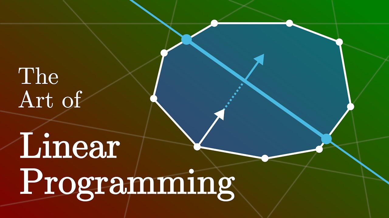
The Art of Linear Programming

MK Kuantitatif - Linier Programming Metode Simpleks
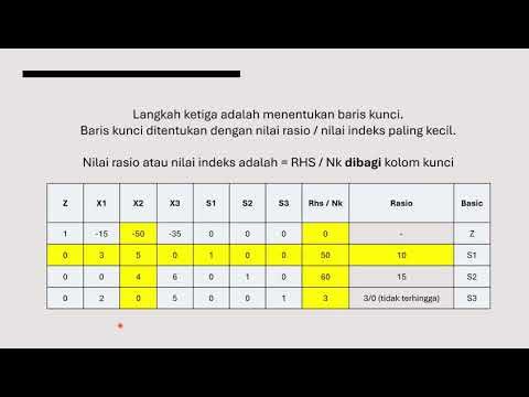
Metode Simplex dengan 3 Variable - Riset Operasional
Riset Operasi #4 - Linear Programming dengan Metode Simpleks | Tutor Manajemen by Gusstiawan Raimanu
5.0 / 5 (0 votes)