Solve Linear Programming (Optimization) Problems in MATLAB - Step by Step Tutorial
Summary
TLDRIn this tutorial, the presenter walks through the process of solving linear programming (LP) problems in Matlab, highlighting key concepts such as formulating the cost function and constraints. The video covers how to translate a given optimization problem into the general form and implement it in Matlab using the 'linprog' function. Key steps include defining vectors, matrices, and optimization options, as well as troubleshooting solutions when constraints are absent. With practical examples and clear instructions, viewers will learn the basics of LP problem-solving and optimization in Matlab, gaining essential skills for mathematical modeling.
Takeaways
- 😀 Learn how to solve linear programming (LP) problems in Matlab using `linprog` function.
- 😀 The tutorial explains the generic form of a linear programming problem, including the cost function and constraints.
- 😀 The cost function is a linear equation that involves a vector of coefficients multiplied by optimization variables.
- 😀 Constraints in LP problems include both equality and inequality constraints, which can be represented in matrix form.
- 😀 The example demonstrates how to transform an optimization problem into Matlab's matrix and vector format.
- 😀 Matlab's `linprog` function can be used with different solvers, such as interior-point, dual simplex, or interior-point legacy.
- 😀 Parameters for the `linprog` function include the maximum number of iterations, optimality tolerance, and constraint tolerance.
- 😀 The tutorial shows how to interpret the solver's output, including the solution vector and the exit flag, to check if the solution is successful.
- 😀 If there are no equality or inequality constraints, you can define them as empty matrices in the `linprog` function.
- 😀 The tutorial encourages viewers to support the channel by liking, subscribing, or donating for continued tutorials.
- 😀 A successful solution is indicated by an exit flag of 1, while any other exit flag suggests issues in the solution process.
Q & A
What is the generic mathematical form of a linear programming problem presented in the tutorial?
-The generic form consists of minimizing a linear cost function f^T x subject to linear inequality constraints A x ≤ b, linear equality constraints Aeq x = beq, and bound constraints lb ≤ x ≤ ub. Here, f is a coefficient vector, x is the vector of optimization variables, A and Aeq are matrices, b and beq are vectors, and lb and ub are lower and upper bound vectors.
Why is the optimization problem considered a linear program?
-It is a linear program because both the cost function and all equality and inequality constraints are linear functions of the decision variables. There are no nonlinear terms such as products or powers of variables.
What does the expression f^T x represent in the context of linear programming?
-The expression f^T x represents the scalar (dot) product between the coefficient vector f and the decision variable vector x. For example, if f = [f1, f2] and x = [x1, x2], then f^T x = f1x1 + f2x2.
What does it mean that the inequality A x ≤ b is applied element-wise?
-Element-wise application means that each row of matrix A multiplied by vector x produces a scalar inequality that must be less than or equal to the corresponding element of vector b. Each row represents a separate constraint.
How are scalar constraints transformed into matrix form?
-Each scalar constraint is rewritten as a row of coefficients multiplied by the variable vector x. These rows are stacked to form matrix A (for inequalities) or Aeq (for equalities), and the right-hand sides form vectors b or beq.
How can the vectors and matrices (f, A, b, Aeq, beq, lb, ub) be determined from a given optimization problem?
-They can be directly read from the reformulated matrix representation of the optimization problem. The coefficients of the objective function form f, the coefficients of inequality constraints form A and b, the coefficients of equality constraints form Aeq and beq, and the variable bounds define lb and ub.
Which MATLAB function is used to solve linear programming problems in the tutorial?
-The MATLAB function used is linprog, which is designed to solve linear programming problems with linear objective functions and linear constraints.
What solver algorithm is selected in the example, and what are some alternative options?
-The interior-point algorithm is selected in the example. Alternative algorithms mentioned include dual-simplex and interior-point-legacy methods.
What optimization options are configured before calling linprog?
-The tutorial configures options such as displaying iteration progress, setting a maximum number of iterations (2000), specifying the optimality tolerance (1e-9), and defining the constraint tolerance (1e-6).
What does the exit flag returned by linprog indicate?
-The exit flag indicates whether the optimization problem was successfully solved. A positive value typically means successful convergence, while zero or negative values indicate that the solver did not successfully find an optimal solution.
What information does the output structure from linprog provide?
-The output structure provides details about the optimization process, such as the algorithm used, iteration count, and other solver-related statistics that describe how the solution was obtained.
How can equality or inequality constraints be removed in MATLAB when solving a linear program?
-To remove equality or inequality constraints, they can be defined as empty matrices (e.g., [] in MATLAB). This tells the solver that those types of constraints do not exist in the problem.
Why does removing constraints typically change the optimal solution?
-Removing constraints enlarges the feasible region, allowing more possible solutions. As a result, the optimal solution and the objective function value may change, often leading to a lower objective value in minimization problems.
What is the key prerequisite for successfully formulating and solving linear programs in MATLAB?
-The key prerequisite is understanding the generic form of linear programming problems and correctly translating the objective function and constraints into vector and matrix form. Without proper formulation, the solver may fail or produce incorrect results.
Outlines

This section is available to paid users only. Please upgrade to access this part.
Upgrade NowMindmap

This section is available to paid users only. Please upgrade to access this part.
Upgrade NowKeywords

This section is available to paid users only. Please upgrade to access this part.
Upgrade NowHighlights

This section is available to paid users only. Please upgrade to access this part.
Upgrade NowTranscripts

This section is available to paid users only. Please upgrade to access this part.
Upgrade NowBrowse More Related Video
Linear Programming Optimization (2 Word Problems)

Solve Linear Program problem in Excel (Solver)

Linear Programming 1: Maximization -Extreme/Corner Points (LP)
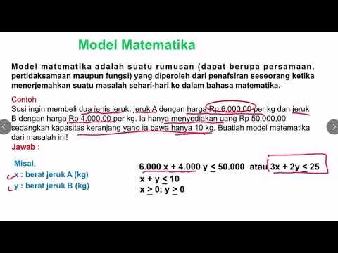
MENENTUKAN MODEL MATEMATIKA DARI SOAL CERITA SPtLDV

Linear Programming dengan Metode Grafik

Tutorial Software POM QM Ep.01 | Program Linear (Linear Programming)
5.0 / 5 (0 votes)