All Learning Algorithms Explained in 14 Minutes

Summary

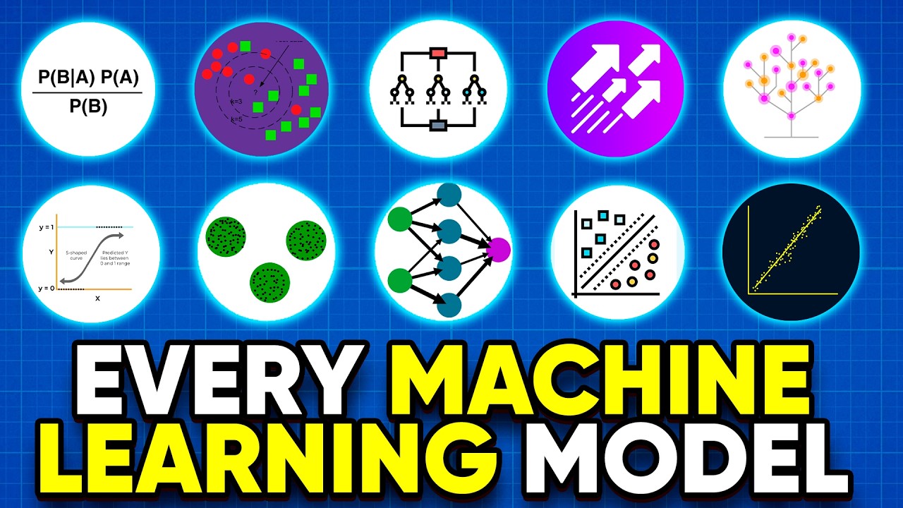
This script offers a comprehensive overview of various machine learning algorithms, including linear regression, support vector machines, naive Bayes, logistic regression, K-nearest neighbors, decision trees, random forests, gradient boosted decision trees, and clustering techniques like K-means, DBSCAN, and PCA. It explains the purpose, methodology, and applications of each algorithm, highlighting their strengths and limitations in solving classification, regression, and clustering tasks.

Takeaways

• 📘 An algorithm is a set of instructions for a computer to perform calculations or problem-solving operations, not an entire program or code.
• 📊 Linear regression is a supervised learning algorithm used to model the relationship between a continuous target variable and one or more independent variables by fitting a linear equation to the data.
• 🛰 Support Vector Machine (SVM) is a supervised learning algorithm used for classification and regression tasks, distinguishing classes by drawing a decision boundary that maximizes the margin from support vectors.
• 🤖 Naive Bayes is a supervised learning algorithm for classification that assumes features are independent and calculates the probability of a class given a set of feature values.
• 📈 Logistic regression is a supervised learning algorithm for binary classification problems, using the logistic function to map input values to a probability between 0 and 1.
• 👫 K-Nearest Neighbors (KNN) is a supervised learning algorithm for both classification and regression that predicts the class or value of a data point based on the majority vote or mean of the closest points.
• 🌳 Decision trees work by iteratively asking questions to partition data, aiming to increase the purity of nodes to make the most informative splits and avoid overfitting.
• 🌲 Random Forest is an ensemble of decision trees that use bagging to reduce the risk of overfitting and improve accuracy through the majority vote or mean values of multiple trees.
• 🌿 Gradient Boosted Decision Trees (GBDT) is an ensemble algorithm that combines individual decision trees in series, with each tree focusing on the errors of the previous one, to achieve high efficiency and accuracy.
• 🔑 K-means clustering is an unsupervised learning method that partitions data into K clusters based on the similarity of data points, using an iterative process to find centroids and assign points to clusters.
• 🏞️ DBSCAN is a density-based clustering algorithm that can find arbitrary shaped clusters and detect outliers without requiring a predetermined number of clusters, using neighborhood distance and minimum points parameters.

Q & A

What is an algorithm in the context of computer science?

An algorithm is a set of commands that a computer must follow to perform calculations or problem-solving operations. It is a finite set of instructions carried out in a specific order to perform a particular task and is not an entire program or code but rather a simple logic to a problem.

How does linear regression model the relationship between variables?

Linear regression models the relationship between a continuous target variable and one or more independent variables by fitting a linear equation to the data. It finds the best regression line by minimizing the sum of squares of the distances between the data points and the line.

What is the primary task of a Support Vector Machine (SVM)?

A Support Vector Machine (SVM) is a supervised learning algorithm primarily used for classification tasks. It distinguishes classes by drawing a decision boundary in multidimensional space, aiming to maximize the distance to support vectors to ensure good generalization.

How does the Naive Bayes algorithm make classification decisions?

The Naive Bayes algorithm, a supervised learning algorithm for classification, assumes that features are independent of each other. It calculates the probability of a class given a set of feature values using Bayes' theorem, relying on the independence assumption to make predictions quickly.

What is the logistic function used for in logistic regression?

The logistic function, also known as the sigmoid function, is used in logistic regression to map any real-valued number to a value between 0 and 1. It is used to perform binary classification tasks by calculating probabilities that can be thresholded to classify data points.

How does the K-Nearest Neighbors (KNN) algorithm determine the class of a data point?

The K-Nearest Neighbors (KNN) algorithm determines the class of a data point based on the majority voting principle of the K closest points. For regression, it takes the mean value of the K closest points, emphasizing the importance of choosing an optimal K value to avoid overfitting or underfitting.

What is the main advantage of decision trees in handling data?

Decision trees have the advantage of being easy to interpret and visualize. They work by iteratively asking questions to partition data, aiming to increase the purity of nodes with each split, which makes them suitable for both classification and regression tasks without the need for feature normalization or scaling.

How does Random Forest differ from a single decision tree?

Random Forest is an ensemble of many decision trees built using bagging, where each tree operates as a parallel estimator. It reduces the risk of overfitting and generally provides higher accuracy than a single decision tree, as it aggregates the results from multiple uncorrelated trees.

What is the boosting method used in Gradient Boosted Decision Trees (GBDT)?

Gradient Boosted Decision Trees (GBDT) use a boosting method that combines individual decision trees sequentially to achieve a strong learner. Each tree focuses on the errors of the previous one, making GBDT highly efficient and accurate for both classification and regression tasks.

How does K-means clustering determine the number of clusters?

K-means clustering does not automatically determine the number of clusters; it requires the number of clusters (K) to be predetermined by the user. The algorithm iteratively assigns data points to clusters and updates centroids until convergence is reached, aiming to group similar data points together.

What are the two key parameters of DBSCAN clustering, and how do they work?

DBSCAN clustering has two key parameters: EPS, which defines the neighborhood distance, and MinPts, which is the minimum number of points required to form a cluster. A point is considered a core point if at least MinPts number of points are within its EPS radius, a border point if fewer points are present, and an outlier if it is not reachable from any core point.

What is the main goal of Principal Component Analysis (PCA)?

The main goal of Principal Component Analysis (PCA) is to reduce the dimensionality of a dataset by deriving new features, called principal components, that explain as much variance within the original data as possible while using fewer features than the original dataset.

Outlines

00:00

🤖 Overview of Machine Learning Algorithms

An algorithm is a set of commands that a computer follows to perform tasks. Linear regression models the relationship between a continuous target variable and independent variables by fitting a linear equation to data, minimizing the sum of squares of distances between data points and the regression line. Support Vector Machines (SVM) draw decision boundaries to classify data, maximizing the distance to support vectors. Naive Bayes, based on Bayes' theorem, assumes feature independence and is fast but less accurate. Logistic regression is used for binary classification, employing a logistic function to map values between 0 and 1. K-Nearest Neighbors (KNN) uses nearby data points to classify or predict values, with optimal K value crucial for avoiding overfitting or underfitting.

05:01

🔍 KNN and Decision Trees

KNN determines the class of a data point based on majority voting of its neighbors, with optimal K value essential to balance specificity and generalization. Decision trees partition data by iteratively asking questions, aiming to increase node purity and predictiveness. Overfitting occurs if the tree becomes too specific, requiring ensemble methods like Random Forests, which use multiple decision trees for improved accuracy and reduced overfitting. Random Forests employ bagging, bootstrapping, and feature randomness to achieve uncorrelated trees and higher accuracy.

10:02

🌲 Boosting and Clustering

Gradient Boosted Decision Trees (GBDT) use boosting to combine weak learners into a strong model, with each tree correcting errors of the previous ones. K-Means clustering partitions data into clusters by iteratively adjusting centroids based on data point distances. DBSCAN clustering finds arbitrary shaped clusters and detects outliers based on density. Principal Component Analysis (PCA) reduces dimensionality by deriving new features that retain most of the original data's variance, often used as a pre-processing step for supervised learning algorithms.

Keywords

💡Algorithm

An algorithm is a set of commands that a computer follows to perform calculations or solve problems. In the context of the video, it refers to various machine learning algorithms used for different tasks like regression, classification, and clustering.

💡Linear Regression

Linear regression is a supervised learning algorithm that models the relationship between a continuous target variable and one or more independent variables by fitting a linear equation to the data. It is illustrated in the video with a chart of data points and a regression line that minimizes the sum of squares of the distances between the points and the line.

💡Support Vector Machine (SVM)

SVM is a supervised learning algorithm used mainly for classification but also for regression tasks. It works by drawing a decision boundary in an N-dimensional space that maximizes the distance to the nearest data points (support vectors). The video explains how SVM handles high-dimensional data efficiently.

💡Naive Bayes

Naive Bayes is a supervised learning algorithm used for classification tasks. It assumes that features are independent, which simplifies computation but can reduce accuracy. The video describes how it uses Bayes' theorem to calculate the probability of a class given a set of features.

💡Logistic Regression

Logistic regression is a supervised learning algorithm used for binary classification problems. It uses the logistic function to map input values to probabilities between 0 and 1, making it suitable for tasks like spam detection and customer churn prediction, as explained in the video.

💡K-Nearest Neighbors (KNN)

KNN is a supervised learning algorithm used for both classification and regression. It determines the class or value of a data point based on the majority class or mean value of its nearest neighbors. The video highlights the importance of choosing an optimal K value to balance specificity and generalization.

💡Decision Tree

A decision tree is a model that uses a tree-like structure to make decisions by asking a series of questions to partition data. The video explains how decision trees can overfit data if they become too specific, and how they are used in ensemble methods like random forests to improve accuracy.

💡Random Forest

Random forest is an ensemble method that combines multiple decision trees using bagging to improve accuracy and reduce overfitting. Each tree is trained on a random subset of the data, and the final prediction is based on the majority vote or average of the trees' predictions. The video describes its advantages over single decision trees.

💡Gradient Boosted Decision Trees (GBDT)

GBDT is an ensemble method that combines decision trees in a sequential manner to correct errors made by previous trees. It is more accurate than random forests but requires careful tuning to avoid overfitting. The video discusses its efficiency in both classification and regression tasks.

💡K-Means Clustering

K-means clustering is an unsupervised learning algorithm that partitions data into K clusters by minimizing the distance between data points and the cluster centroids. The video explains the iterative process of selecting centroids, assigning points to clusters, and recalculating centroids until convergence.

Highlights

An algorithm is a finite set of instructions for a computer to perform calculations or problem-solving operations.

Linear regression models the relationship between a continuous target variable and one or more independent variables by fitting a linear equation to the data.

Support Vector Machine (SVM) is used for classification and regression tasks by drawing a decision boundary to distinguish classes.

SVM maximizes the distance to support vectors when drawing the decision boundary to avoid sensitivity to noise and improve generalization.

Naive Bayes classifier assumes feature independence and uses Bayes' theorem for classification tasks.

Logistic regression is used for binary classification problems and is based on the logistic function to map real values to a probability between 0 and 1.

K-Nearest Neighbors (KNN) algorithm determines the class of a data point based on the majority voting principle of the closest points.

Choosing an optimal K value in KNN is crucial to avoid overfitting or underfitting.

Decision trees partition data by asking iterative questions and are prone to overfitting without proper ensemble techniques.

Random Forest is an ensemble of decision trees that reduces the risk of overfitting and improves accuracy.

Gradient Boosted Decision Trees (GBDT) combines individual decision trees using boosting methods for efficient and accurate predictions.

K-means clustering is an unsupervised learning method that groups data points based on similarities and requires the number of clusters to be predetermined.

DBSCAN is a density-based clustering algorithm that can find arbitrary shaped clusters and is robust to outliers.

Principal Component Analysis (PCA) is a dimensionality reduction technique that derives new features to retain significant variance with fewer dimensions.

PCA is widely used as a preprocessing step for supervised learning algorithms to enhance performance.

The order of principal components in PCA is determined by the fraction of variance they explain.

Each machine learning algorithm has unique characteristics and applications, making them suitable for different types of problems and data sets.

Transcripts

every single machine learning algorithm

explained in case you don't know an

algorithm is a set of commands that must

be followed for a computer to perform

calculations or like other

problemsolving operations according to

its formal definition an algorithm is a

finite set of instructions carried out

in a specific order to perform a

particular task it's not an entire

program or code it is simple logic to a

problem linear regression is a

supervised learning algorithm and tries

to model their relationship between a

continuous Target variable and one or

more independent VAR variables by

fitting a linear equation to the data

take this chart of dots for example a

linear regression model tries to fit a

regression line to the data points that

best represents the relations or

correlations with this method the best

regression line is found by minimizing

the sum of squares of the distance

between the data points and the

regression line so for these data points

the regression line Looks like this

support Vector machine or svm for short

is a supervised learning algorithm and

is mostly used for classification tasks

but is also suitable for regression R

tasks svm distinguishes classes by

drawing a decision boundary how to draw

or determine the decision boundary is

the most critical part in svm algorithms

before creating the decision boundary

each observation or data point is

plotted in N dimensional space with n

being the number of features used for

example if we use length and width to

classify different cells observations

are plotted in a two-dimensional space

and decision boundary is a line if we

use three features decision boundary is

a plane in three-dimensional space if we

use more than three features decision

boundary becomes a hyper plane which is

really hard to visualize decision

boundary is drawn in a way that the

distance to support vectors are

maximized if the decision boundary is

too close to a support Vector it'll be

highly sensitive to noises and not

generalize well even very small changes

to independent variables may cause a

misclassification svm is especially

effective in cases where number of

dimensions are more than the number of

samples when finding the decision

boundary svm uses a subset of training

points rather than all points which

makes it memory efficient on the other

hand training time increases for large

data sets which negatively affects the

performance Nave Bas is a supervised

learning algorithm used for

classification tasks hence it is also

called Nave Bas classifier Nave Bas

assumes that features are independent of

each other and there is no correlation

between features however this is not the

case in real life this Nave Assumption

of features being uncorrelated is the

reason why this algorithm is called

naive the intuition behind naive Bay

algorithm is the Bas theorem p a is the

probability of event a given event B has

already occurred PBA is probability of

event B given event a has already

occurred PA is the probability of event

a and PB is the probability of event B

naive Bas classifier calculates the

probability of a class given a set of

feature values the the assumption that

all features are independent makes knif

based algorithm very fast when compared

to complicated algorithms in some cases

speed is preferred over higher accuracy

but on the other hand the same

assumption makes knife Bas algorithm

less accurate than complicated

algorithms logistic regression is a

supervised learning algorithm which is

mostly used for binary classification

problems logistic regression is a simple

yet very effective classification

algorithm so it is commonly used for

many binary classification tasks things

like customer turn spam email website or

ad click predictions are some examples

of the areas where logistic regression

offers a powerful solution the basis of

logistic regression is the logistic

function also called the sigmoid

function which takes any real value

number and Maps it to a value between 0o

and 1 Let's consider we have the

following linear equation to solve

logistic regression model takes a linear

equation as input and uses logistic

function and log odds to perform a

binary classification task then we will

get the f famous shaped graph of

logistic regression we can use the

calculated probability as is for example

the output can be the probability that

this email is Spam is 95% or the

probability that the customer will click

on the ad is 70% however in most cases

probabilities are used to classify data

points for example if the probability is

greater than 50% the prediction is

positive class or one otherwise the

prediction is negative class or zero K

nearest Neighbors or K&N for short is a

supervised learning algorithm that can

be used to solve both classification and

regression tasks the main idea behind

KNN is that the value of a class or of a

data point is determined by the data

points around it KNN classifier

determines the class of a data point by

majority voting principle for instance

if K is set to five the classes of five

closest points are checked prediction is

done according to the majority class

similarly K&N regression takes the mean

value of five CL closest points let's go

over an example consider the following

data points that belong to four

different classes and let's see how the

predicted classes change according to

the K value it is very important to

determine an optimal K value if K is too

low the model is too specific and not

generalized well it also tends to be too

sensitive to noise the model

accomplishes a high accuracy on train

set but will be a poor predictor on new

previously unseen data points therefore

we are likely to end up with an overfit

model on the the other hand if K is too

large the model is too generalized and

is not a good predictor on both train

and test sets this situation is known as

underfitting KNN is simple and easy to

interpret it does not make any

assumption so it can be implemented in

nonlinear tasks KNN does become very

slow as number of data points increases

because the model needs to store all

data points thus it is not memory

efficient another downside of KNN is

that it is sensitive to outliers

decision trees work by iteratively

asking questions to partition data it is

easier to conceptualize the partitioning

data with a visual representation of a

decision tree this represents a decision

tree to predict customer CH first split

is based on monthly charges amount then

the algorithm keeps asking questions to

separate class labels the question get

more specific as the tree gets deeper

the aim is to increase the

predictiveness as much as possible at

each partitioning so that the model

keeps gaining information about the data

set randomly splitting the feature does

not usually give us the valuable insight

into the data set it's the splits that

increase purity of nodes that are most

informative the purity of a node is

inversely proportional to the

distribution of different classes in

that node the questions to ask are

chosen in a way that increases Purity or

decreases impurity but how many

questions do we ask when do we stop when

is our tree sufficient to solve our

classification problem the answer to all

of these questions leads us to one of

the most important Concepts in machine

learning overfitting the model can keep

asking questions until all nodes are

pure however this would be a two

specific model and would not generalize

will it achieves high accuracy with

training set but performs poorly on new

previously unseen data points which

indicates overfitting decision tree

algorithm usually does not require to

normalize or scale features it is also

suitable to work on a mixture of feature

data types on the negative side it is

prone to overfitting and needs to be

ensembled in order to generalize well

random Forest is an ensemble of many

decision trees random forests are built

using a method called bagging in which

decision trees are used as par parel

estimators if used for a classification

problem the result is based on majority

vote of the results received from each

decision tree for regression the

prediction of a leaf node is the mean

value of the target values in that leaf

random Forest regression takes mean

values of results from decision trees

random forests reduce the risk of

overfitting and accuracy is much higher

than a single decision tree furthermore

decision trees in a random forest run in

parallel so that the time does not

become a bottleneck the success of a

random Forest highly depends on using

uncorrelated decision trees if we use

the same or very similar trees the

overall result will not be much

different than the result of a single

decision tree random forests achieve to

have uncorrelated decision trees by

bootstrapping and feature Randomness

bootstrapping is randomly selecting

samples from training data with

replacement they are called the

bootstrap samples feature Randomness is

achieved by selecting features randomly

for each decision Tree in a random

Forest the number of features used for

each tree in a random Forest can be

controlled with maxcore features

parameter random Forest is a highly

accurate model on many different

problems and does not require

normalization or scaling however it is

not a good choice for high dimensional

data sets compared to fast linear models

gradient boosted decision trees or gbdt

for short is an ensemble algorithm which

uses boosting methods to combine

individual decision trees boosting means

combining a learning algorithm in series

to achieve a strong learner from many

sequentially connect weak Learners in

the case of gbdt the weak Learners are

the decision trees each tree attempts to

minimize the errors of previous tree

trees in boosting are weak learners but

adding many trees in series and each

focusing on the errors from the previous

one make boosting a highly efficient and

accurate model unlike bagging boosta

does not involve bootstrap sampling

every time a new tree is added it fits

on a modified version of the initial

data set since trees are added

sequentially boosting algorithms learn

slowly in statistical learning models

that learn slowly perform better gbdt is

very efficient on both classification

and regression tasks and provides more

accurate predictions compared to random

Forest it can handle mixed type of

features and no pre-processing is needed

gbdt does require careful tuning of

hyperparameters in order to prevent the

model from overfitting K means

clustering clustering is a way to group

a set of data points in a way that

similar data points are grouped together

therefore clustering algorithms look for

similarities or dissimilarities among

data points clustering is an

unsupervised learning method so there is

no label associated with data points

clustering algorithms try to find the

underlying structure of the data

observations or data points in a

classification task have labels each

observation is classified according to

some measurements classification

algorithms try to model the relationship

between measurements on observations and

their assigned class then the model

predicts the class of new observations K

means clustering aims to partition data

into K clusters in a way that data

points in the same cluster are similar

and data points in different clusters

are further apart thus it is a partition

based clustering technique similarity of

two points is determined by the distance

between them consider the following 2D

visualization of a data set it can be

partied into four different clusters now

real life data sets are much more

complex in which clusters are not

clearly separated however the algorithm

works in the same way K means is an

iterative process it is built on

expectation maximization algorithm after

the number of clusters are determined it

works by executing the following steps

number one it randomly selects the

centroids or the center of cluster for

each cluster then it calculates the

distance of all data points to the

centroids it assigns the data points to

the closest cluster it finds the new

centroids of each cluster by taking the

mean of all data points in the cluster

and it repeats steps 2 3 and four until

all points converge and cluster Center

stop moving K means clustering is

relatively fast and easy to interpret it

is also able to choose the positions of

initial centroids in a smart way that

speeds up the convergence the one

challenge with K means is that the

number of clusters must be predetermined

cayman's algorithm is not able to guess

how many clusters exist in the data if

there is a nonlinear structure

separating groups in the data K means

will not be a good choice DB scan

clustering partition based and

hierarchical clustering techniques are

highly efficient with normal shaped

clusters however when it comes to

arbitrary shaped clusters or detecting

outliers density based techniques are

more efficient DB scan stands for

density based spatial clustering of

applications with noise it is able to

find arbitrary shaped clusters and

clusters with noise the main idea behind

DB scan is that a point belongs to a

cluster if it is close to many points

from that cluster there are two key

parameters of DB scan EPS which is the

distance that specifies the neighborhood

two points are considered to be

neighbors if the distance between them

are less than or equal to EPs and Min

pts which is the minimum number of data

points to define a cluster based on

these two parameters points are

classified as score Point border point

or outlier a point is a core point if

there are at least Min pts number of

points including the point itself in its

surrounding area with radius EPS a point

is a border point if it is unreachable

from a core point and there are less

than Min pts number of points within its

surrounding area and a point is an

outlier if it is not a core point and

not reach from any core points DB scan

does not require to specify a number of

clusters beforehand it is robust to

outliers and able to detect the outliers

in some cases determining an appropriate

distance of neighborhood EPS is not easy

and it requires domain knowledge

principle components analysis or PCA is

a dimensionally reduction algorithm

which basically derives new features

from the existing ones with keeping as

much information as possible PCA is an

unsupervised learning algorithm but it

is also widely used as a pre-processing

step for supervised learning algorithms

PCA deres new features by finding the

relations among features in a data set

the aim of PCA is to explain the

variance within the original data set as

much as possible by using less features

the new derived features are called

principal components the order of

principal components is determined

according to the fraction of variance of

original data set they explain the

advantage of PCA is that a significant

amount of variance of the original data

set is retained using much smaller

number of features than the original

data set principal components are

ordered according to the amount of

variants that they explain and that is

every common machine learning algorithm

explained