Matrix multiplication as composition | Chapter 4, Essence of linear algebra
Summary
TLDRThis educational video script delves into the concept of linear transformations and their representation through matrices. It explains how these transformations can be visualized as altering space while maintaining grid lines' parallelism and even spacing, with the origin fixed. The script emphasizes that a linear transformation is determined by the effect on basis vectors, like i-hat and j-hat in two dimensions. It then illustrates how matrix multiplication represents applying one transformation after another, highlighting the importance of order in such operations. The script uses examples to clarify the geometric interpretation of matrix multiplication and introduces the concept of matrix composition, demonstrating its computation and reinforcing the idea with visual aids. It concludes by advocating a conceptual understanding of matrix operations over rote memorization, promising to extend these concepts beyond two dimensions in a future video.
Takeaways
- 📚 Linear transformations are represented by matrices, which map vectors to vectors while preserving the structure of space.
- 📏 Linear transformations can be visualized as 'smooshing' space without altering the parallelism and spacing of grid lines, with the origin fixed.
- 🎯 The outcome of a linear transformation on any vector is determined by the transformation's effect on the basis vectors (i-hat and j-hat in 2D).
- 📈 A vector's new position after a transformation can be found by multiplying its original coordinates with the new coordinates of the basis vectors.
- 📋 The coordinates where the basis vectors land after a transformation are recorded as the columns of a matrix, which defines matrix-vector multiplication.
- 🔄 The composition of two linear transformations results in a new transformation that can be represented by a matrix formed by the final positions of i-hat and j-hat.
- 🔢 Matrix multiplication geometrically represents the sequential application of one transformation followed by another, read from right to left.
- 🔄 Understanding matrix multiplication through the lens of transformations can simplify complex concepts and proofs, such as associativity.
- 🧩 The order of matrix multiplication matters because different sequences of transformations can lead to distinct outcomes.
- 📉 The example of applying a shear followed by a rotation versus a rotation followed by a shear demonstrates the importance of the order of operations.
- 🌐 Associativity in matrix multiplication is intuitively understood as applying a series of transformations in the same sequence, regardless of grouping.
Q & A
What is a linear transformation?
-A linear transformation is a function that takes vectors as inputs and produces vectors as outputs, preserving the operations of vector addition and scalar multiplication. It can be visually thought of as 'smooshing' space in a way that grid lines remain parallel and evenly spaced, with the origin fixed.
How are linear transformations represented using matrices?
-Linear transformations are represented using matrices by recording the coordinates where the basis vectors (like i-hat and j-hat in two dimensions) land after the transformation. These coordinates become the columns of the matrix, and matrix-vector multiplication is used to compute the transformation of any vector.
Why are basis vectors important in linear transformations?
-Basis vectors are important because any vector in the space can be described as a linear combination of these basis vectors. Knowing where the basis vectors land after a transformation allows us to determine where any other vector will land.
What is the geometric consequence of linear transformations keeping grid lines parallel and evenly spaced?
-The geometric consequence is that after a transformation, a vector with coordinates (x, y) will land at x times the new coordinates of i-hat plus y times the new coordinates of j-hat, maintaining the linear relationship between input and output vectors.
How does matrix multiplication relate to applying one linear transformation after another?
-Matrix multiplication geometrically represents the composition of two linear transformations. You first apply the transformation represented by the matrix on the right, and then apply the transformation represented by the matrix on the left.
What is the composition matrix and how is it formed?
-The composition matrix is a matrix that captures the overall effect of applying one linear transformation after another as a single action. It is formed by determining the final locations of the basis vectors after both transformations and using these locations as the columns of the new matrix.
How does the order of matrix multiplication affect the result?
-The order of matrix multiplication is significant because it represents applying one transformation after another in a specific sequence. Changing the order can result in a completely different transformation, as the effect of each transformation on the basis vectors will be different.
Why is matrix multiplication considered associative?
-Matrix multiplication is associative because applying three transformations in the order of A then B then C will have the same effect regardless of whether you first combine A with B or B with C. This is intuitive when thinking of transformations being applied sequentially.
What does it mean to multiply a matrix by a vector?
-Multiplying a matrix by a vector means applying the linear transformation represented by the matrix to the vector. This is done by taking the dot product of the matrix's rows (or columns) with the vector, resulting in a new vector that represents the transformed input vector.
How can understanding matrix multiplication as transformations help with learning?
-Understanding matrix multiplication as applying one transformation after another provides a conceptual framework that makes the properties of matrix multiplication more intuitive and easier to grasp, rather than just memorizing the mathematical process.
What is the significance of the convention of recording the coordinates of i-hat and j-hat landing as matrix columns?
-Recording the coordinates where i-hat and j-hat land as matrix columns standardizes the representation of linear transformations. It allows for a systematic way to compute the transformation of any vector through matrix-vector multiplication.
Outlines

This section is available to paid users only. Please upgrade to access this part.
Upgrade NowMindmap

This section is available to paid users only. Please upgrade to access this part.
Upgrade NowKeywords

This section is available to paid users only. Please upgrade to access this part.
Upgrade NowHighlights

This section is available to paid users only. Please upgrade to access this part.
Upgrade NowTranscripts

This section is available to paid users only. Please upgrade to access this part.
Upgrade NowBrowse More Related Video

Lecture 61: Linear Algebra (Matrix representations of linear transformations)
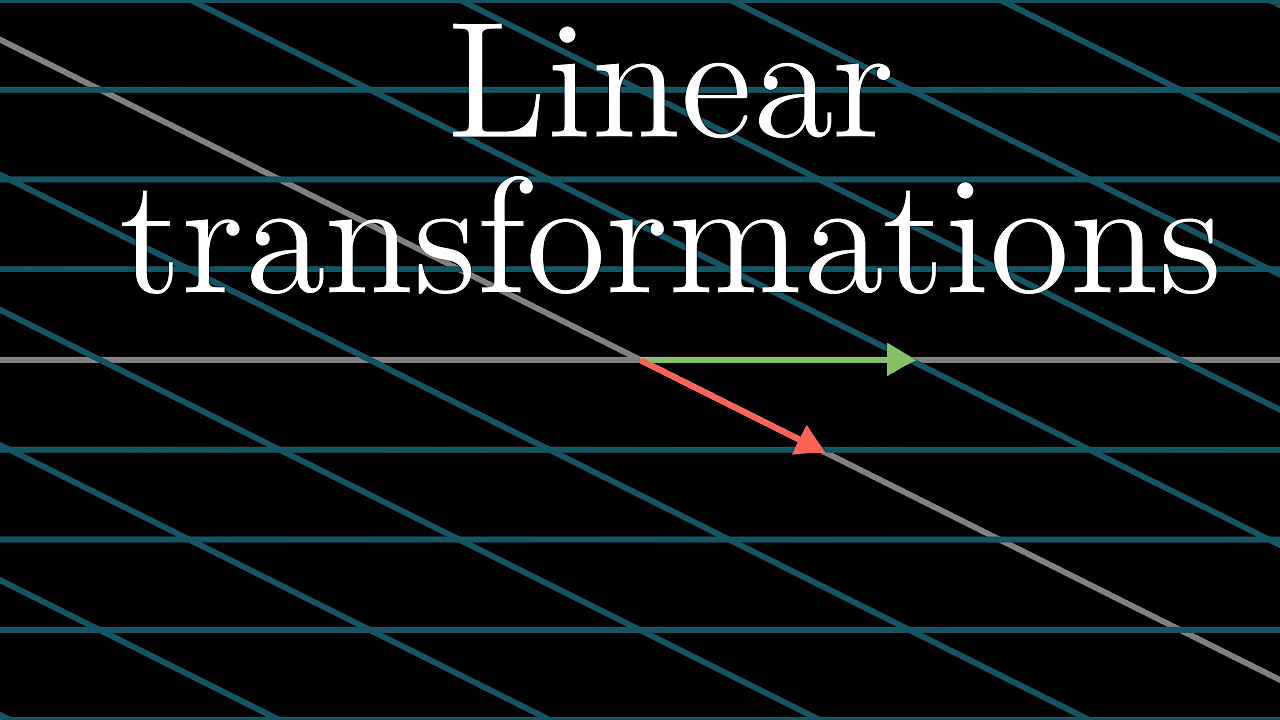
Linear transformations and matrices | Chapter 3, Essence of linear algebra
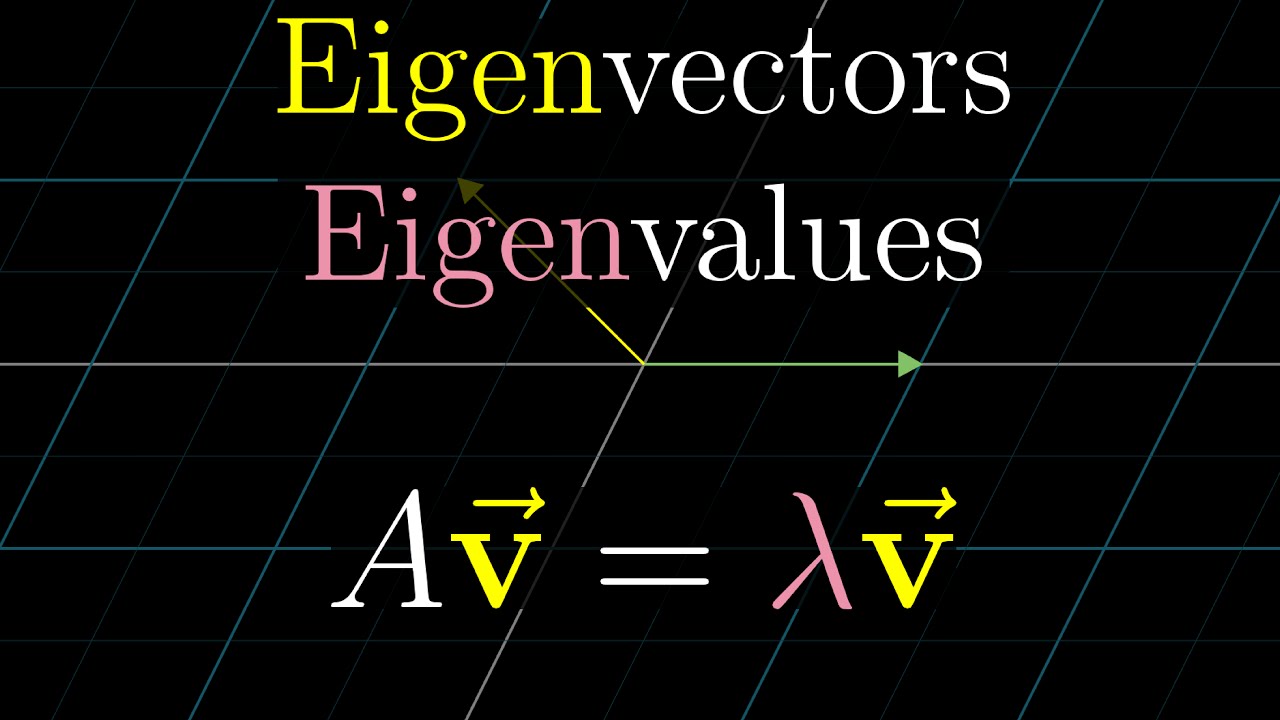
Eigenvectors and eigenvalues | Chapter 14, Essence of linear algebra

Aljabar Linier - Ruang Hasil Kali Dalam - Perubahan Basis

Matrices for General Linear Transformations | Linear Algebra
Transformasi Geometri Bagian 5 -Transformasi Matriks Matematika Wajib Kelas 11
5.0 / 5 (0 votes)