Kinematics Part 1: Horizontal Motion
Summary
TLDRProfessor Dave introduces the concept of horizontal motion in classical physics, focusing on kinematics, which describes motion without considering forces. He explains that kinematics, developed by Galileo, uses equations to predict the motion of objects in one and two dimensions. The video covers three fundamental kinematic equations involving displacement, velocity, acceleration, and time, and demonstrates their application to real-world examples, such as calculating velocity and distance traveled for a car accelerating from rest and stopping from a given velocity. The summary emphasizes the simplicity and universality of these equations, applicable to all objects on Earth and in space, and invites viewers to subscribe for more educational content.
Takeaways
- 📚 Classical physics is divided into kinematics and dynamics, focusing on the motion of objects without and with forces, respectively.
- 🌟 Kinematics was largely developed by Galileo in the early 1600s, breaking away from Aristotle's view of imperfect earthly motion.
- 🔢 Kinematic equations involve variables for displacement, velocity, acceleration, and time, with constant acceleration in this context.
- 📉 Subscript 'zero' after velocity or displacement indicates initial conditions, which are crucial for solving problems.
- ⚙️ The three fundamental kinematic equations relate velocity, position, and acceleration to time and initial conditions.
- 🚗 Additional equations help define average velocity and position in terms of time intervals and final/initial velocities.
- 🛣️ Real-world examples, such as driving to the supermarket, demonstrate how to apply kinematic equations to find velocity and distance traveled.
- 🏎️ For a car accelerating from rest, velocity after time 't' can be found by multiplying acceleration by time, and distance by using the kinematic equation for position.
- 🚑 In the case of braking, the time to stop and the braking distance can be calculated using the same set of kinematic equations.
- 🔁 The kinematic equations are universally applicable to any object in motion, not just cars.
- 📈 Understanding and applying these equations allows for the prediction of motion under various conditions, showcasing the power of classical mechanics.
Q & A
What are the two main branches of mechanics in classical physics?
-The two main branches of mechanics in classical physics are kinematics and dynamics.
Who is credited with largely developing kinematics?
-Galileo is credited with largely developing kinematics in the early 1600s.
What is the primary focus of kinematics?
-Kinematics focuses on equations that describe the motion of objects without reference to forces of any kind.
How does dynamics differ from kinematics?
-Dynamics is the study of the effect that forces have on the motion of objects, unlike kinematics which does not consider forces.
What was the common belief about mathematical descriptions of motion before Galileo?
-Before Galileo, it was believed that mathematics could only describe the perfect motion of divine celestial objects and that the motion of objects on earth was too imperfect and unpredictable to calculate.
What are the variables included in the kinematic equations?
-The kinematic equations include variables for displacement, velocity, acceleration, and time.
Why is acceleration considered to have a constant value in kinematics?
-In kinematics, acceleration is considered to have a constant value because the study does not look at forces that could cause acceleration to change over time.
What does the subscript of zero after velocity or displacement indicate?
-The subscript of zero after velocity or displacement indicates initial conditions, which have implications depending on the problem being analyzed.
What are the three fundamental kinematic equations mentioned in the script?
-The three fundamental kinematic equations are: 1) velocity at any time T is equal to initial velocity plus acceleration times time, 2) position with respect to a point of origin is equal to initial position plus initial velocity times time plus one-half the acceleration times time squared, and 3) velocity squared is equal to initial velocity squared plus twice the acceleration times displacement.
What are the two supplemental equations derived from simple definitions in kinematics?
-The two supplemental equations are: position is equal to the average velocity times the time interval, and the average velocity is equal to final velocity plus initial velocity over 2.
How can the kinematic equations be applied to calculate the velocity and distance traveled by a car accelerating at a constant rate?
-The kinematic equations can be applied by plugging in known values such as initial velocity, acceleration, and time to calculate the final velocity and distance traveled. For example, if a car starts from rest and accelerates at 2.5 m/s² for 10 seconds, its velocity would be 25 m/s and it would have traveled 125 meters.
How can you determine the time it takes for a moving car to stop and the distance it travels while braking?
-You can determine the time it takes for a car to stop by using the equation that relates final velocity, initial velocity, and acceleration. Once you have the time, you can use another equation to find the braking distance by plugging in the initial velocity, acceleration, and time.
How does the script demonstrate the universality of kinematic equations?
-The script demonstrates the universality of kinematic equations by showing that they can be applied to any object, not just cars, and that they govern the motion of all objects whether on earth or in space.
Outlines

This section is available to paid users only. Please upgrade to access this part.
Upgrade NowMindmap

This section is available to paid users only. Please upgrade to access this part.
Upgrade NowKeywords

This section is available to paid users only. Please upgrade to access this part.
Upgrade NowHighlights

This section is available to paid users only. Please upgrade to access this part.
Upgrade NowTranscripts

This section is available to paid users only. Please upgrade to access this part.
Upgrade NowBrowse More Related Video
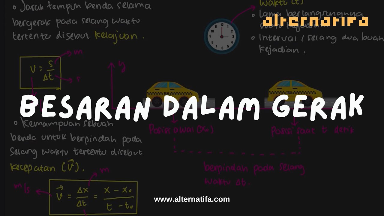
Kinematika Gerak : Besaran dalam Gerak | Fisika SMA | Alternatifa

FISIKA KINEMATIKA KELAS XI JARAK PERPINDAHAN KELAJUAN KECEPATAN PART 1 KURIKULUM MERDEKA

MATERI KINEMATIK kelas 11 bag 1 PENGERTIAN GERAK, JARAK & PERPINDAHAN K Merdeka

mod01lec03 - Introduction to Mobile Robot Kinematics

Tebongkar! Rahasia Cepat Memahami Kinematika Gerak dengan jelas dan detail! (Seri Fisika Dasar)
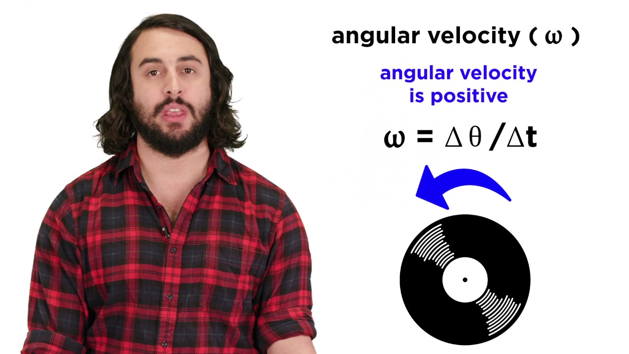
Angular Motion and Torque
5.0 / 5 (0 votes)