FEA V29: Gaussian Quadrature

Schuster Engineering
25 May 201711:21

Summary

TLDRThis video script delves into Gaussian quadrature, a pivotal method for numerical integration in finite element analysis. It explains how Gaussian quadrature is used to calculate the stiffness matrix by integrating over an element's volume. The script highlights the importance of the Jacobian determinant in transforming integrals from global to local coordinates. It also discusses the properties of the B matrix and the challenges of integrating ratios of polynomials. The script further illustrates how Gaussian quadrature efficiently approximates integrals of polynomial functions with fewer function evaluations, providing examples of single, double, and triple integration points for increasing accuracy. Finally, it applies Gaussian quadrature to evaluate a nodal force vector, demonstrating the trade-off between accuracy and computational efficiency.

Takeaways

  • πŸ“ Gaussian quadrature is a method for numerical integration used in finite element analysis.
  • 🌐 The isoparametric stiffness matrix is calculated by integrating over the volume of an element using B transpose times D times B.
  • πŸ” The Jacobian determinant is key in transforming integrals from global to local coordinates, simplifying the process.
  • πŸ“ The limits for the natural coordinates s and t in numerical integration typically range from -1 to 1.
  • πŸ“ˆ B matrices depend on nodal positions, making each element's B matrix distinct in the global system.
  • πŸ”’ Good elements have linear terms in B and B transpose, leading to quadratic expressions when multiplied.
  • πŸ“‰ Poor quality elements can result in complex ratios of polynomials for the Jacobian determinant, complicating integration.
  • πŸ“‹ Gaussian quadrature is efficient for polynomial integrands, requiring fewer function evaluations for the same accuracy.
  • πŸ“Š The method involves evaluating the function at specific locations (integration points) and multiplying by interval widths for area approximation.
  • πŸ“‰ Using more integration points increases accuracy but also the computational cost, as it requires more function evaluations.
  • πŸ”§ An example demonstrates the difference between single and two-point Gaussian quadrature, with the latter providing exact results for quadratic functions.

Q & A

  • What is Gaussian quadrature?

    -Gaussian quadrature is a method for numerical integration that is particularly efficient for polynomial integrands. It approximates the integral of a function by evaluating it at specific points (integration points) and multiplying by weights, which are determined to minimize the number of evaluations needed for a given level of accuracy.

  • Why is Gaussian quadrature important in finite element analysis?

    -In finite element analysis, Gaussian quadrature is crucial for calculating the stiffness matrix of each element in a structure. It allows for the transformation of the integration from the global coordinate system to the natural coordinate system, simplifying the process and making it computationally efficient.

  • What is the significance of the Jacobian determinant in Gaussian quadrature?

    -The Jacobian determinant is significant because it relates the infinitesimal areas in the global coordinate system to the natural coordinate system. It is used to transform the limits of integration from global to local coordinates, which simplifies the integration process in finite element analysis.

  • How does the quality of an element affect the integration process?

    -The quality of an element affects the integration process because it influences the complexity of the integrand. Good quality elements have simpler integrands, often polynomials, which are easier to integrate using Gaussian quadrature. Poor quality elements may have more complex integrands, such as ratios of polynomials, which are harder to integrate.

  • What are the properties of the B matrices in the context of Gaussian quadrature?

    -The B matrices in Gaussian quadrature depend on the nodal positions and are used to map from the natural to the global coordinate system. Each B matrix is distinct for each element because it depends on the element's nodal positions. The B matrices are defined in terms of natural coordinates s and t.

  • How does the number of integration points affect the accuracy of Gaussian quadrature?

    -The number of integration points in Gaussian quadrature directly affects the accuracy of the numerical integration. More points generally provide higher accuracy, especially for higher-degree polynomial integrands. However, it also increases the computational cost, as more function evaluations are required.

  • What is the role of the integration points in Gaussian quadrature?

    -Integration points in Gaussian quadrature are the specific locations at which the function is evaluated. These points are chosen to optimize the accuracy for polynomial integrands. The choice of these points, along with the interval width, determines the efficiency and accuracy of the numerical integration.

  • Why is it beneficial to evaluate the function at the midpoint in a single integration point scenario?

    -Evaluating the function at the midpoint in a single integration point scenario is beneficial because it provides an exact result for linear integrands. This is due to the property that a linear function will average out to zero over a symmetric interval, resulting in an exact integral value.

  • How does the width of the rectangles in Gaussian quadrature relate to the number of integration points?

    -The width of the rectangles in Gaussian quadrature changes with the number of integration points. With more points, the rectangles may have different widths, with the central rectangle often being wider to give more emphasis to the central region of the integration range, which is especially important for higher-degree polynomials.

  • What is the practical example given in the script for using Gaussian quadrature?

    -The practical example given in the script is the evaluation of a nodal force vector in a finite element model. The script explains how Gaussian quadrature can be used to approximate the integral of a quadratic function to find the force vector, with different levels of accuracy depending on the number of integration points used.

  • What is the difference between one-point and two-point Gaussian quadrature integration?

    -One-point Gaussian quadrature integration evaluates the function at the midpoint of the interval and is exact for linear integrands. Two-point integration evaluates the function at two specific points and is exact for cubic integrands. The two-point method is more accurate for quadratic integrands compared to the one-point method.

Outlines

00:00

πŸ“ Introduction to Gaussian Quadrature in Finite Element Analysis

The first paragraph introduces Gaussian Quadrature as a method for numerical integration, particularly crucial in finite element analysis. It explains that every element in a structure requires a stiffness matrix, which necessitates integration over the element's volume. The paragraph then delves into the isoparametric stiffness matrix, detailing how it's calculated through integration over the volume of B transpose times D times B. It highlights the use of the Jacobian determinant to transform the integral from global to local coordinates, simplifying the process by integrating over natural coordinates s and t. The discussion then shifts to the properties of the integral, emphasizing the dependency of the B matrices on nodal positions and the implications of element quality on the complexity of the integral. It concludes by setting the stage for Gaussian Quadrature as an efficient method for numerical integration, especially suited for polynomial integrands.

05:00

πŸ“Š Gaussian Quadrature for Polynomial Integration

This paragraph explains how Gaussian Quadrature works in practice, focusing on its application for polynomial integrands. It describes the process of approximating an integral as the sum of rectangular areas, where the width and height of the rectangles are determined by specific mathematical formulas. The paragraph illustrates the concept with examples of single, double, and triple integration points, showing how the number and position of these points affect the accuracy of the integration. It emphasizes the importance of evaluating the function at specific locations, known as integration points, to achieve optimal results. The discussion also touches on the practical implications of function evaluation in terms of computational efficiency, especially when dealing with large matrices in finite element analysis. The paragraph concludes with an example of using Gaussian Quadrature to evaluate a nodal force vector, demonstrating the method's accuracy and efficiency.

10:01

πŸ” Accuracy of Gaussian Quadrature in Polynomial Integration

The third paragraph provides a detailed analysis of the accuracy of Gaussian Quadrature, particularly when dealing with polynomial functions of varying degrees. It contrasts the results of single-point and two-point integration with the actual value of a quadratic function to illustrate the method's effectiveness. The paragraph explains how single-point integration can lead to significant errors for non-linear integrands, while two-point integration provides exact results for up to cubic integrands. It further discusses the implications of these findings for the evaluation of nodal force vectors in finite element analysis, emphasizing the importance of choosing the right number of integration points to ensure accuracy. The paragraph concludes by setting the stage for further discussion on the application of Gaussian Quadrature in two-dimensional elements and the calculation of stiffness matrices.

Mindmap

Keywords

πŸ’‘Gaussian Quadrature

Gaussian Quadrature is a method used for numerical integration, which is a technique to calculate the integral of a function. It is particularly useful for finite element analysis where elements require integration over their volume to form stiffness matrices. The video explains that Gaussian Quadrature is efficient for polynomial integrands, meaning it can approximate the area under a curve with fewer function evaluations. It is used to evaluate integrals in the context of calculating the stiffness matrix of elements in a structure.

πŸ’‘Numerical Integration

Numerical Integration is the process of calculating an integral using numerical methods, which is a key concept in the video. It is necessary when analytical methods are not feasible. The video discusses how Gaussian Quadrature is used to perform numerical integration in the context of finite element analysis, specifically for calculating the integral over the volume of an element.

πŸ’‘Isoparametric Stiffness Matrix

The Isoparametric Stiffness Matrix is a matrix used in finite element analysis to represent the stiffness of an element. The video mentions that this matrix is calculated by integrating over the volume of an element. Gaussian Quadrature is used to perform this integration numerically, which is crucial for constructing the stiffness matrix in the global coordinate system.

πŸ’‘Jacobian Determinant

The Jacobian Determinant is a scalar value resulting from the determinant of the Jacobian matrix, which relates the infinitesimal volumes in local and global coordinate systems. The video explains that the Jacobian determinant is used to transform differential areas from global to local coordinates, which simplifies the integration process in the context of finite element analysis.

πŸ’‘Shape Functions

Shape Functions are mathematical functions used in finite element analysis to describe the shape of an element. They are used to map coordinates from the local to the global system. The video discusses how the B matrix, which is part of the stiffness matrix calculation, is derived from the shape functions and nodal positions.

πŸ’‘Nodal Positions

Nodal Positions refer to the coordinates of the nodes in a finite element model. The video explains that each element's B matrix is distinct because it depends on the nodal positions of the element. These positions are crucial for mapping from the natural to the global coordinate system.

πŸ’‘Integration Points

Integration Points are the specific locations at which the function is evaluated in Gaussian Quadrature. The video illustrates that choosing the right integration points is essential for achieving accurate results with fewer function evaluations. It shows how single, two, and three-point integration can be used for different levels of accuracy.

πŸ’‘Bilinear Quadrilateral Element

A Bilinear Quadrilateral Element is a type of element in finite element analysis that uses bilinear shape functions. The video mentions that for such elements, both B and B transpose will have linear terms in s and t, leading to a quadratic expression when multiplied. This is important for understanding the complexity of the integrals involved in the stiffness matrix calculation.

πŸ’‘Polynomial Integrands

Polynomial Integrands are functions that are polynomials, which are integrals of polynomial functions. The video highlights that Gaussian Quadrature is particularly efficient for polynomial integrands. It shows how the method can achieve exact results for up to a certain degree of polynomial by choosing the right number of integration points.

πŸ’‘Distributed Force

Distributed Force refers to a force that is distributed over an area or volume. The video provides an example of how Gaussian Quadrature can be used to evaluate a nodal force vector due to a distributed force. It shows the calculation process and how numerical integration can be applied to find the force at a node.

πŸ’‘Isoparametric Element

An Isoparametric Element is a type of element in finite element analysis that uses the same shape functions for both geometry and field variables. The video discusses how the stiffness matrix for an isoparametric element is calculated using numerical integration, specifically Gaussian Quadrature.

Highlights

Gaussian quadrature is introduced as a method for numerical integration.

Gaussian quadrature is crucial for finite element analysis in structural engineering.

The stiffness matrix is derived through integration over the element's volume.

The Jacobian determinant is used to transform integrals from global to local coordinates.

The stiffness matrix in the global system is calculated by integrating over local coordinates.

The B matrices are defined in terms of natural coordinates s and t.

The limits for s and t in numerical integration range from -1 to 1 for a 2x2 square element.

The B matrices depend on nodal positions, making each element's B matrix distinct.

Good quality elements have linear terms in B and B transpose, resulting in quadratic expressions.

Poor quality elements can have polynomial ratios in the Jacobian determinant, complicating integration.

The determinant of the Jacobian is constant for good elements, simplifying the integration process.

Gaussian quadrature is an efficient method for polynomial integrands, requiring fewer function evaluations.

The integration points in Gaussian quadrature are chosen to optimize results for polynomials.

A single integration point is used for linear integrands, providing an exact result.

Two integration points are used for quadratic and cubic integrands, also providing exact results.

Three integration points are used for higher accuracy, particularly for fifth degree polynomial integrands.

The number of function evaluations is critical due to the computational cost of evaluating matrices.

An example is provided where Gaussian quadrature is used to evaluate a nodal force vector.

Single point integration is exact for linear integrands but not for quadratic integrands.

Two point integration is exact for cubic integrands and should be accurate for quadratic functions.

The video concludes with an example of using Gaussian quadrature for 2D isoparetric elements.

Transcripts

play00:00

this video introduces gaussian

play00:02

quadrature as a method for numerical

play00:05

integration

play00:06

gaussian quadrature is an important tool

play00:08

for numerical integration in finite

play00:10

element analysis because every every

play00:13

single element in a structure requires a

play00:15

stiffness Matrix and to get to that

play00:18

stiffness Matrix you need to integrate

play00:19

over the volume of the element so

play00:21

focusing on the isoparametric stiffness

play00:23

Matrix we know that it's equal to the

play00:26

integral over the volume of B transpose

play00:28

times D times B

play00:30

but in terms of the isoparametric we

play00:33

have the B's defined in terms of s and t

play00:36

and the element in global coordinates in

play00:39

terms of X and Y

play00:41

what we can do though is

play00:43

use the property of the Jacobian

play00:46

determinant which is that it's equal to

play00:48

the ratio of the areas Global to local

play00:51

so in in infinitesimal areas that just

play00:56

means that the determinant of the

play00:57

Jacobian is equal to dxdy divided by DS

play01:00

DT or in other words we can substitute

play01:02

dxdy for Jacobian times dsdt

play01:07

so that's what we do here that gives us

play01:09

an equation for the stiffness Matrix

play01:12

which is going to be the stiffness

play01:14

Matrix in the global system directly but

play01:17

we get to integrate over the local

play01:19

coordinate system the natural

play01:20

coordinates of s and t and the nice

play01:22

thing about that is first of all the B's

play01:25

and the J are all defined in terms of s

play01:27

and t but secondarily the limits for S

play01:30

and T both go from negative one to one

play01:32

because it's this two by two square

play01:34

element this is the integral we now want

play01:37

to solve using numerical integration

play01:40

before we get into the integration

play01:42

itself let's talk about a few properties

play01:44

of this integral first off the B

play01:46

matrices in here depend on the nodal

play01:49

positions the B Matrix we developed in a

play01:52

prior video we used the shape functions

play01:56

times the nodal positions in order to

play01:58

give us a mapping from the natural to

play02:01

the global system and in that process we

play02:05

were able to calculate the B Matrix so

play02:07

every B Matrix is distinct for each

play02:10

element in the global system because it

play02:12

depended on those element Noble

play02:14

positions

play02:15

for a good element a good bilinear

play02:18

quadrilateral element or Q4 both B and B

play02:22

transpose will have linear terms if s

play02:24

and t so when you multiply B and B

play02:26

transpose you're going to get a

play02:27

quadratic expression but poor quality

play02:31

elements because the determinant of the

play02:33

Jacobian enters into B so we're going to

play02:36

be dividing by that twice and then

play02:38

multiplying it by it again

play02:40

um

play02:41

we're going to end up with ratios of

play02:42

polynomials so poor quality element will

play02:45

have a polynomial for the determinant of

play02:47

the Jacobian so we're going to be

play02:49

dividing by that

play02:51

this means that we're going to have an

play02:55

issue potentially doing the integration

play02:57

because a ratio of polynomials is much

play02:59

more complex to integrate than just a

play03:02

single polynomial however for good

play03:04

elements the determinant of the Jacobian

play03:06

is constant

play03:08

for lower quality it's going to be a

play03:10

quadratic term so our real question here

play03:12

is what can we do to allow the Fe code

play03:15

for every single element to go through

play03:17

this integral and evaluate it it will be

play03:20

a different integral for every single

play03:21

one what do we do well we turn to

play03:23

numerical integration this is what the

play03:26

background is the reason that we want to

play03:28

do gaussian quadrature

play03:30

so what is gaussian quadrature well

play03:32

first off quadrature is just another

play03:34

term for numerical integration it is a

play03:36

way of approximating the integral or the

play03:38

area under a curve of a function with

play03:41

the sum of rectangular areas like what's

play03:43

shown here gaussian quadrature in

play03:45

particular is designed to be unlike the

play03:47

Vermont sums which are generic designed

play03:50

to be a most efficient approach for

play03:53

polynomial integrands so you evaluate

play03:56

the function fewer times to get the same

play03:59

level of accuracy and remember that good

play04:01

quality quadrilateral elements have

play04:03

quadratic integrands so they are

play04:05

polynomials in gaussian quadrature what

play04:07

we do is we change the number and the

play04:10

width of the intervals in order to get

play04:11

the accuracy that we desire for a given

play04:14

polynomial also the height of the

play04:16

rectangle is not evaluated right at the

play04:18

midpoint such as in shown in the figure

play04:20

above it's actually going to be

play04:22

evaluated at a specific location chosen

play04:25

to give us optimal results for

play04:27

polynomials and that location is called

play04:30

the integration point for the interval

play04:32

and finally the choice of the interval

play04:35

width and that evaluation point is what

play04:37

gives us a very efficient minimizing the

play04:40

number of evaluations a method of

play04:42

getting an accurate result for a

play04:44

polynomial

play04:45

let's see how this works in practice

play04:47

let's imagine for instance that we have

play04:49

a function such as shown on the screen

play04:51

that's a function of s where s is going

play04:54

to vary from negative 1 to 1 and we find

play04:56

want to find the integral of this

play04:57

function on that range

play05:00

so this is what we're trying to solve

play05:02

for what we do with gaussian quadrature

play05:04

is that we approximate this as the sum

play05:07

of a series of rectangles where W

play05:10

represents the width of the rectangle

play05:12

and F of s i is the height of the

play05:15

rectangle at a specific location s i

play05:18

so if we want to do a single integration

play05:21

point then what we're going to do is

play05:23

evaluate the function smack dab in the

play05:25

middle and multiply by the width of the

play05:27

rectangle which is just going to be 2.

play05:29

so height of or S1 is evaluated at zero

play05:34

so F of 0 and then the width of the

play05:37

rectangle is 2.

play05:39

that gives us an exact result for any

play05:42

linear integrand as you might expect you

play05:45

evaluate at one point it's going to

play05:47

average out negative on one side

play05:48

positive and the other or above and

play05:50

below we will get an exact result

play05:52

however obviously for the function shown

play05:54

here it's not a great approximation

play05:58

well what if we want something more

play05:59

accurate well we can go to two

play06:01

integration points so we have the same

play06:03

function here and again we're going to

play06:05

approximate it as the sum of rectangles

play06:09

but now we're going to apply two

play06:10

rectangles as shown here and we're going

play06:13

to evaluate those rectangles not smack

play06:15

in the middle of the range but at

play06:17

specific locations in particular when we

play06:20

go from -1 to 1 the first location is is

play06:23

at minus 1 over the square root of 3 and

play06:26

the second is as plus 1 over the square

play06:28

root of 3. so when I evaluate at those

play06:32

locations that's minus 0.577 and plus

play06:35

0.577 then the width of each rectangle

play06:38

is going to be equal to 1 and that's

play06:41

what gives me the equation shown here

play06:44

where I'm evaluating each the function

play06:46

at two locations plus and minus 0.577

play06:50

this gives me an exact result for up to

play06:54

a cubic integrand so quadratic and cubic

play06:57

would both give exact results for two

play07:00

integration points over the range of

play07:02

negative one to one

play07:04

taking it one step further if you really

play07:07

if you want to get even more accurate

play07:08

how about three integration points in

play07:10

other words evaluating with three

play07:12

rectangles here's where we're going to

play07:14

see that we want to actually change the

play07:16

width of the rectangles you can see here

play07:18

the middle rectangle ends up being extra

play07:21

emphasized it's a wider rectangle again

play07:24

this is for a polynomial that's what

play07:26

you'd want to have is the center section

play07:28

to be more important than the outer two

play07:31

and what we're going to do is evaluate

play07:34

the left hand section which has a width

play07:37

of 5 9. we're going to evaluate at a

play07:39

position again from the negative one to

play07:41

one range its first position is minus

play07:45

0.774 and then the middle section is a

play07:49

wider width so that's 8 9 and it's

play07:53

evaluated right where the

play07:55

s is equal to zero

play07:58

and then the last piece is again back to

play08:00

5 9 and it's evaluated at a positive

play08:02

0.774

play08:04

this gives me an exact result for up to

play08:07

a fifth degree polynomial integround so

play08:10

it's a pretty darn accurate result

play08:11

especially if you've got polynomial

play08:13

integrounds for just three evaluations

play08:15

of your function now you notice I'm keep

play08:17

talking about this evaluation of the

play08:19

function and that's important because it

play08:22

takes computer time to evaluate the

play08:25

function remember the function here is

play08:26

actually a big Matrix that we're

play08:28

evaluating and we're doing it on every

play08:30

single element so if you have to

play08:31

evaluate that Matrix one location that's

play08:35

a lot less time than say three locations

play08:39

here well it's a third of the time

play08:42

let's wrap up this video with a quick

play08:44

example of using gaussian quadrature to

play08:48

evaluate a nodal Force Vector in a prior

play08:51

video I showed you how to find the force

play08:53

Vector for the distributed Force shown

play08:55

the t y here and we ended up with an

play08:57

expression that looked like this where

play08:59

we had shape function 1 and shape

play09:01

function four each evaluated at the

play09:03

position where s is equal to negative 1

play09:05

and Y is equal to 2. so here I'm

play09:08

actually evaluating with T is my

play09:11

variable but again the range is from

play09:12

negative one to one

play09:14

so when I

play09:16

um multi when I plug in the value for or

play09:20

the expression for N1 and N4 we end up

play09:23

with an integral at Node 1 in the y

play09:26

direction that looks like this

play09:28

um that's the integral that we now want

play09:30

to use gaussian quadrature to evaluate

play09:32

so first of all let's go back to if I

play09:35

evaluate that integral directly because

play09:36

obviously I can it's a simple polynomial

play09:39

I get 83.3 pounds as my Force so if now

play09:43

I decide to approximate that with a

play09:46

single integration point which is going

play09:48

to be exact up to a linear integrand

play09:51

notice this is a quadratic integrand so

play09:53

it will not be exact

play09:55

so at one point integration means I take

play09:57

the full width of the integral from

play09:59

negative 1 to 1 in the T Direction so

play10:01

that's 2 and then I multiply it by the

play10:03

function evaluated in the middle of the

play10:05

range so that's at location 0.

play10:07

so that gives me this expression when I

play10:10

plug in t equal to 0 in the inside the

play10:12

integrand and it gives me a final total

play10:15

of 62.5 pounds that's a 25 error by

play10:19

using a single point integration

play10:21

let's try the two point integration

play10:23

which should be exact up to cubic and

play10:25

since this is a quadratic function it

play10:27

should give me the exact result

play10:29

so again here I'm evaluating it with two

play10:32

rectangles each rectangle has a width of

play10:35

one and I'm evaluating at negative one

play10:38

over the square root of 3 and positive 1

play10:40

over the square root of 3. where T is my

play10:43

my variable that is plus or minus 1 over

play10:46

square root of T of 3. plugging that

play10:49

into my expression with the integrand I

play10:52

get 83.3 pounds so I have no error

play10:55

present when I do the two point

play10:57

integration and that's what I expect

play10:58

because this is just a quadratic

play11:00

function so that's just a small example

play11:03

of using this in the next video I'll go

play11:05

through what we do for two dimensional

play11:08

elements and then we'll take to take

play11:10

that to an example to find the stiffness

play11:12

Matrix using both one point and two

play11:16

point integration on a 2d isoparetric

play11:19

element

Rate This
β˜…
β˜…
β˜…
β˜…
β˜…

5.0 / 5 (0 votes)

Related Tags
Numerical IntegrationGaussian QuadratureFinite Element AnalysisStiffness MatrixIsoparametric ElementsJacobian DeterminantShape FunctionsPolynomial IntegrandsEngineering MathematicsNumerical Methods