How AI Image Generators Work (Stable Diffusion / Dall-E) - Computerphile
Summary
TLDRThis transcript explores the inner workings of image generation using diffusion models, contrasting them with traditional generative adversarial networks (GANs). It delves into the process of adding and removing noise in images to gradually reconstruct an image from random noise. The explanation covers various technical aspects, such as the iterative process of predicting and subtracting noise, along with how text embeddings can guide image generation. The discussion also touches on practical applications, including tools like Stable Diffusion and the use of Google Colab for running these models. The video concludes with insights into how these models can be accessed and used for image creation.
Takeaways
- 😀 Diffusion models generate images by iteratively removing noise, starting with random noise and refining it step by step into a clear image.
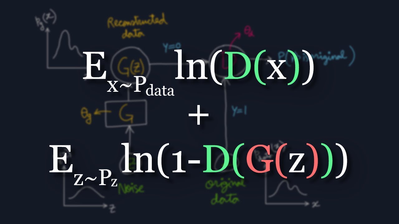
- 😀 GANs (Generative Adversarial Networks) involve two networks: a generator that creates images and a discriminator that distinguishes between real and fake images.
- 😀 Training GANs can be challenging due to issues like mode collapse, where the generator produces repetitive or limited outputs.
- 😀 Diffusion models offer a more stable alternative to GANs by gradually refining noisy images, making them easier to train.
- 😀 In diffusion models, the network is trained to predict the noise added to an image during training, which is then reversed during generation.
- 😀 Diffusion models require several steps of noise addition and removal, making them more computationally expensive than some other generative models.
- 😀 The process of generating images with diffusion models involves conditioning the model with specific inputs like text descriptions (e.g., 'frog on stilts').
- 😀 Classifier-free guidance helps steer the model's output by running two versions of the model: one with text conditioning and one without, then amplifying the difference between them.
- 😀 Generative models like diffusion models can be used in platforms like Google Colab, which allows users to experiment with models like Stable Diffusion for free, with paid options for higher compute power.
- 😀 While diffusion models are powerful for generating high-quality images, they still face challenges with controlling and fine-tuning the output to match specific conditions.
- 😀 The ability to condition diffusion models with text prompts and adjust the generation process makes them versatile and applicable for creative image generation tasks.
Q & A
What are the primary differences between GANs and diffusion models in image generation?
-GANs (Generative Adversarial Networks) consist of two networks: a generator and a discriminator. The generator creates fake images while the discriminator evaluates them. This process can suffer from issues like mode collapse and instability. In contrast, diffusion models start with noise and gradually refine it to produce a clear image. They are more stable and less prone to issues like mode collapse, making them suitable for high-quality image generation.
How do diffusion models work in terms of generating images from noise?
-Diffusion models work by gradually adding noise to an image and then training a model to reverse this process. The model learns to predict and remove the noise at each step, progressively refining an image from pure noise to a final, coherent result. This iterative process helps create high-quality images.
What role does classifier-free guidance play in image generation with diffusion models?
-Classifier-free guidance enhances the specificity of the generated image by conditioning the model on input, like text descriptions. It adjusts the noise prediction to ensure that the generated image is closely aligned with the given prompt. This allows for more control over the generated output, leading to images that more accurately reflect the input conditions.
What is the significance of using text embeddings in diffusion models?
-Text embeddings are crucial because they allow the diffusion model to condition image generation on textual descriptions. By converting the text into a numerical representation (embedding), the model uses this information to guide the generation process, ensuring the final image aligns with the given prompt.
How does the training process for diffusion models differ from that of GANs?
-In GANs, the generator and discriminator compete, with the generator trying to create realistic images while the discriminator tries to differentiate between real and fake images. This can result in instability and challenges in generating high-quality images. In diffusion models, training involves adding noise to images and teaching the model to reverse the noise process. This approach is more stable and doesn't face the same challenges as GANs.
Why is stability an important advantage of diffusion models over GANs?
-Stability is a significant advantage of diffusion models because it leads to more reliable image generation. GANs can struggle with mode collapse and instability during training, making it harder to generate diverse and high-quality images. Diffusion models avoid these issues by focusing on a gradual process of noise removal, leading to more predictable results.
Can diffusion models be used for tasks beyond image generation?
-Yes, diffusion models are not limited to just image generation. They can be adapted for other tasks like audio synthesis and video generation. The underlying principle of gradually refining noisy input can be applied to various domains, making diffusion models a versatile tool.
How accessible are diffusion models for everyday users, and what platforms can they use?
-Diffusion models are increasingly accessible thanks to platforms like Google Colab, which allow users to run these models for free, albeit with limited resources. This enables users to experiment with image generation and other tasks without needing extensive computational resources.
What challenges do users face when trying to generate high-quality images using diffusion models?
-While diffusion models are more stable than GANs, generating high-quality images can still be computationally intensive. Users may face limitations in terms of processing power, especially when using platforms like Google Colab, which provide limited access to hardware like GPUs. Fine-tuning models for specific tasks can also be challenging for beginners.
How do iterative processes in diffusion models contribute to generating high-quality images?
-The iterative process in diffusion models involves refining an image over multiple steps. Starting with pure noise, the model progressively removes the noise, improving the image’s clarity and quality with each iteration. This gradual refinement helps ensure that the final image is high-resolution and detailed.
Outlines

This section is available to paid users only. Please upgrade to access this part.
Upgrade NowMindmap

This section is available to paid users only. Please upgrade to access this part.
Upgrade NowKeywords

This section is available to paid users only. Please upgrade to access this part.
Upgrade NowHighlights

This section is available to paid users only. Please upgrade to access this part.
Upgrade NowTranscripts

This section is available to paid users only. Please upgrade to access this part.
Upgrade Now


5.0 / 5 (0 votes)