36. Regressione: bontà d'adattamento

Summary

The transcript discusses the process of finding the regression line that represents the average dependence of y on x. It then explores evaluating the fit of this regression line to observed data through the concept of deviation of ypsilon, which is the sum of the squared differences between observed and mean values of y. The deviation is further broken down into regression deviation and error deviation. The script explains how to calculate the index of determination (R-squared) to assess the model's fit, which ranges from 0 to 1, indicating a perfect fit when equal to 1 and a poor fit when close to 0. The speaker also covers alternative methods for calculating regression deviation and provides examples to illustrate these concepts.

Takeaways

• 📉 The regression line represents the average dependency of y on x.
• 🔍 The goodness of fit for a regression line evaluates how well the model represents observed data.
• ➗ Total deviance of y can be split into regression deviance and error deviance.
• 📏 The coefficient of determination (R²) is used to assess the fit of the regression model.
• 0️⃣ If R² is close to 0, the model is poor; if it’s 1, the model is perfect.
• 🔺 Deviance of regression can be calculated with a simpler formula involving xy covariance.
• 🧮 R² is the proportion of variability in y explained by x; in one example, it was 61%.
• ⚠️ The model might explain only a part of the variability, with other factors influencing the rest.
• 📊 In a weighted case, the deviance of regression is calculated differently but follows similar principles.
• 🤔 A low R² suggests the model does not fit well, with much of the variability attributed to other factors.

Q & A

What is the purpose of the regression line in the context of the script?

The regression line, or the line of regression, is used to express the average dependency of the variable 'y' on the independent variable 'x'. It represents the trend of the relationship between the two variables.

How is the goodness of fit of the regression line assessed?

The goodness of fit is assessed by examining the deviation of 'ypsilon' (the dependent variable) from the mean of 'y'. This is broken down into two components: the regression deviation and the error deviation.

What does the regression deviation represent?

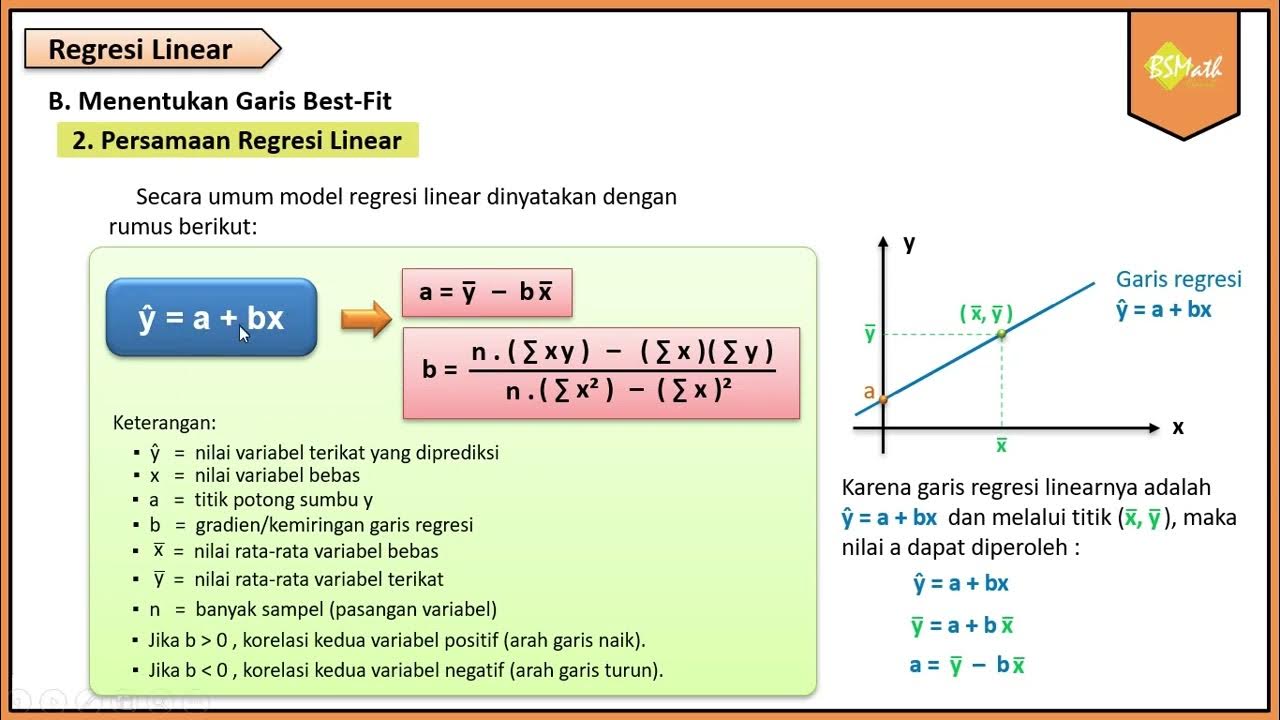
The regression deviation is the sum of the squared differences between the predicted values ('y hat') and the mean of 'y'. It measures how well the regression line fits the data points.

What is meant by the error deviation in the script?

The error deviation is the sum of the squared differences between the actual values of 'y' and the predicted values ('y hat'). It represents the part of the variation in 'y' that is not explained by the regression line.

How is the total deviation of 'ypsilon' calculated?

The total deviation of 'ypsilon' is calculated by summing the squared differences between each observed 'y' value and the overall mean of 'y'.

What is the significance of the determination index (R-squared) in the script?

The determination index, often denoted as R-squared, is a measure of how well the regression line fits the data. It is calculated as the ratio of the regression deviation to the total deviation of 'ypsilon'. It varies between 0 and 1, with values closer to 1 indicating a better fit.

What does an R-squared value of 0 indicate about the regression model?

An R-squared value of 0 indicates that the regression model is not suitable for representing the observed phenomenon, meaning the regression line does not fit the data at all.

How is the alternative formula for calculating the regression deviation used?

The alternative formula for calculating the regression deviation involves the product of the sum of the cross-deviations of 'x' and 'y' divided by the sum of the deviations of 'x'. This method can be more convenient when dealing with a large number of data points.

What is the interpretation of an R-squared value of 0.61 as mentioned in the script?

An R-squared value of 0.61 suggests that the linear relationship between 'y' (the dependent variable) and 'x' (the independent variable) explains 61% of the variability in 'y'. This indicates that the regression model fits the data reasonably well.

How does the script differentiate between the simple and weighted cases in regression analysis?

The script differentiates between the simple and weighted cases by adjusting the formulas for calculating the regression deviation and the determination index to account for the weights assigned to each data point in the weighted case.

What is the coefficient of correlation squared mentioned in the script?

The coefficient of correlation squared refers to the square of the Pearson correlation coefficient, which is used to measure the strength and direction of the linear relationship between two variables. In the context of regression analysis, it is equivalent to the R-squared value.

Outlines

00:00

📊 Understanding Regression Analysis

This paragraph introduces the concept of regression analysis, specifically focusing on the calculation of the regression line that represents the average dependency of 'y' on 'x'. It discusses the goodness of fit of the regression line, which is a measure of how well the regression line represents the observed phenomenon. The paragraph explains the concept of total deviation (devianza di ypsilon), which can be broken down into regression deviation (devianza di regressione) and error deviation (devianza d'errore). The regression deviation is calculated as the sum of the squared differences between the observed 'y' values and their mean, while the error deviation is the sum of the squared differences between the observed 'y' values and the values predicted by the regression line. The paragraph also describes how to visually represent these concepts using a scatter plot with the regression line and the mean line for 'y'.

05:02

🔢 Calculating the Coefficient of Determination

The second paragraph delves into the calculation of the coefficient of determination, often denoted as R-squared, which is a measure of how well the regression model fits the data. It explains that R-squared is calculated as the ratio of the regression deviation to the total deviation. The paragraph provides a step-by-step calculation of R-squared using both the full formula and a simplified version. It also discusses the interpretation of R-squared values, indicating that a value close to 1 suggests a perfect fit, while a value close to 0 indicates a poor fit. The paragraph concludes with an example calculation, demonstrating how to compute the R-squared value for a given dataset and interpret its meaning in the context of the linear relationship between 'y' (savings per year) and 'x' (number of family members).

10:07

📉 Exploring Weighted Regression and Alternative Calculation Methods

The third paragraph extends the discussion to weighted regression, where the data points have different weights, and introduces an alternative method for calculating the regression deviation. It explains the formula for the weighted regression coefficient and how to calculate the weighted regression deviation. The paragraph also covers the concept of the coefficient of correlation and its square, which is related to the coefficient of determination. It provides an example of how to calculate the regression deviation using the alternative formula, which involves the sum of the product of 'x' and 'y' values, divided by the deviation of 'x'. The paragraph concludes by emphasizing the importance of understanding different calculation methods for regression analysis and the interpretation of the coefficient of determination in the context of the linear relationship between 'y' (annual expenditure) and 'x' (annual income).

Keywords

💡Regression Line

The regression line, also known as the line of best fit, is a straight line that represents the average relationship between two variables. In the video, it is used to express the dependency of 'y' on 'x'. The regression line is calculated to minimize the distance between the observed values and the predicted values, which helps in understanding the trend of the data.

💡Goodness of Fit

Goodness of fit refers to how well a statistical model represents the observed data. In the context of the video, it is used to evaluate the effectiveness of the regression line in representing the observed phenomenon. The video discusses how to verify the goodness of fit by examining the deviation of 'y' from the regression line.

💡Deviance

Deviance, in the context of regression analysis, is a measure of how far the observed values are from the values predicted by the model. The video explains that the total deviance of 'y' can be decomposed into two parts: the regression deviance and the error deviance. This concept is crucial for understanding the model's accuracy.

💡Regression Deviance

Regression deviance is the part of the total deviance that is attributed to the regression model. It is calculated as the sum of the squared differences between the observed values and the values predicted by the regression line. The video uses this concept to illustrate how the regression line fits the data.

💡Error Deviance

Error deviance, also known as residual deviance, is the part of the total deviance that is not explained by the regression model. It represents the inherent variability in the data that the model does not account for. The video discusses how this is calculated and its significance in evaluating the model's performance.

💡Index of Determination (R-squared)

The index of determination, often denoted as R-squared, is a statistical measure that represents the proportion of the variance in the dependent variable that is predictable from the independent variable(s). The video explains how to calculate R-squared and interpret its value to assess the quality of the regression model.

💡Coefficient of Determination

The coefficient of determination is another term for the index of determination and is used interchangeably in the video. It is a key indicator of how well the regression model fits the data. A higher value indicates a better fit, while a lower value suggests that the model does not explain much of the variability in the data.

💡Residuals

Residuals are the differences between the observed values and the values predicted by the regression model. In the video, residuals are used to calculate the error deviance and are essential for diagnosing the fit of the regression model. The discussion of residuals helps in understanding the discrepancies between the model's predictions and the actual data.

💡Scatter Plot

A scatter plot is a type of plot that shows the relationship between two variables. In the video, a scatter plot is used to visualize the data points and the regression line, helping to illustrate the linear relationship between 'y' and 'x'. The scatter plot is a fundamental tool for regression analysis.

💡Weighted Deviance

Weighted deviance is a concept that extends the idea of deviance to situations where data points have different weights or importance. The video mentions this in the context of calculating deviance in a weighted regression model, which is a more advanced topic in statistical analysis.

💡Correlation Coefficient

The correlation coefficient is a measure of the strength and direction of the linear relationship between two variables. The video hints at the relationship between the index of determination and the square of the correlation coefficient, indicating that a higher correlation implies a better fit of the regression model.

Highlights

Exploring the function that expresses the regression line, which on average shows the dependence of y on x.

Verifying the goodness of fit of the regression line to determine its utility in representing the observed phenomenon.

Introducing the concept of deviation of epsilon (ε) as a measure to evaluate the regression line's fit.

Differentiating between the deviation of regression and the deviation of error in the context of epsilon's deviation.

Graphical representation of the dispersion graph with the regression line and the mean line for y.

Calculating the total deviation of ypsilon as the sum of squared differences from the mean of y.

Defining the regression deviation as the sum of squared differences between predicted and mean values of y.

Describing the error deviation as the sum of squared differences between observed and predicted values on the regression line.

Evaluating the model's fit to the data using the coefficient of determination (R-squared).

Interpreting the coefficient of determination in terms of the model's ability to represent the observed phenomenon.

Calculating the coefficient of determination using the formula involving total, regression, and error deviation.

Discussing the implications of an R-squared value close to 0 or 1 and its impact on the model's effectiveness.

Providing a step-by-step calculation of the coefficient of determination for a given dataset.

Comparing the calculated R-squared value to assess the model's fit and its practical implications.

Exploring an alternative formula for calculating the regression deviation and its practical use.

Discussing the weighted case for calculating the regression deviation and its significance.

Highlighting the importance of the coefficient of determination in understanding the model's explanatory power.

Explaining the relationship between the coefficient of correlation and the coefficient of determination.

Transcripts

2 abbiamo visto come trovare la funzione

che esprime la retta di regressione è

quindi che esprime in media la

dipendenza di y da ics ora verifichiamo

la bontà di adattamento di questa retta

di aggressione cioè verifichiamo se e

quanto è utile questa retta di

regressione a rappresentare il fenomeno

osservato consideriamo la devianza di

ypsilon che sarà uguale da sommato re

delle elezioni in meno una media di y al

quadrato

questa devianza ti possiamo scomporre in

due devianze alla devianza di

regressione e la devianza terrore quindi

la devianza di ypsilon sarà uguale a

devianza di aggressioni più devianza

d'errore la devianza di regressione è

uguale la sommatoria delle azioni

cappello meno y medio al quadrato

la doglianza d'errore è uguale alla

sommatoria delle elezioni meno y il

cappello al quadrato

quindi riprendiamo il grafico precedente

quindi del caso semplice abbiamo il

grafico di dispersione rappresentato

dalla linea nera la retta di regressione

rappresentata dalla rossa è questa linea

blu che invece rappresenta la media di

ypsilon che era uguale a 5 di 25 per cui

la media di ypsilon è rappresentata come

una linea una retta che è parallela

all'asse delle ips dunque la devianza di

ypsilon è data dalla sommatoria delle

differenze tra la ypsilon i è la media

generale di y al quadrato

quindi è dato dalla sommatoria di queste

distanze qui tra punto osservato

edizioni alla media di y la somma di

queste quattro distanze che sto

indicando con il mouse al quadrato

mi davate fidanzati y

ovviamente la casa di ypsilon è uguale

alla devianza di regressione più la

devianza terrore per cui può essere

scomposta come la somma delle distanze

tra i punti teorici sulla retta di

regressione è la media generale di y

quindi la somma di queste quattro

distanze al quadrato

mi dà la devianza di aggressione

la tendenza delle loro invece è dato

dalla sommatoria delle distanze tra il

valore osservato inizio è il valore

teorico sulla retta di regressione

quindi come possiamo vedere la devianza

di ypsilon è uguale a pat alianza di

repressione più la devianza terrore

quindi detto questo valutiamo la bontà

riadattamento del modello di regressione

ai dati osservati attraverso l'indice di

determinazione che viene spesso con r

quadro che è uguale alla devianza di

regressione tv isolate nyanza di y

dato che devianza di ypsilon è uguale a

davis di regressione più difese delle

ore la devianza di regressione che può

essere scritta in questo modo piazzati

si sono meno devianza terrore per cui

possiamo sostituire al numeratore

tendenza di repressione con questa

formula devianza di un meno devianza

terrore avrò degli alzati y meno

devianza terrore diviso devianza di y

uguale degli altri e condiviso devianza

di ypsilon che vuole a uno meno devianza

per loro è diviso devianza di y ed è

quadro varia tra 0 e 1 serve quadro ora

zero allora significa che è il modello è

pessimo cioè non è adatto a

rappresentare il fenomeno osservato ad

esempio questo è un caso in cui r4 si

approssima 0 di uguale a 0,00 19 in

questo caso infatti la retta di

regressione non è adatta a rappresentare

la dipendenza in media di y taix i fatti

quel grafico ha degli alti e bassi per

cui sarebbe impossibile rappresentarlo

perfettamente con una retta

quindi in questo caso il modello di

regressione quindi la retta di

regressione per modello si intende

proprio una retta di repressione è

pessimo quando era il quadro invece

uguale a 1 il modello è perfetto quindi

la resa di aggressione e passa

esattamente

per i valori osservati quindi le

edizioni saranno uguali alla ypsilon

cappello coni per cui la devianza di

regressione sarà uguale alla terrazza di

ypsilon e la devianza terrore sarà

uguale a zero in quanto in questo caso

non commettiamo nessun errore

tracciando la retta di regressione

vediamo come calcolare l'indice

determinazione abbiamo il caso per caso

considerato il caso che abbiamo visto in

precedenza va da casa di ypsilon è data

dalla formula semplice sommatoria delle

elezioni meno la mente di siamo al

quadrato

faremo anche calcolarla con la formula

ridotta e la stessa cosa quindi tre meno

5 vivo 25 al quadrato

più sei meno 5,25 quadrato più 5 meno

5,25 quadrato più 7 meno 52 25 al

quadrato è uguale a 8,75 la devianza di

aggressioni invece potevo calcolare

facendo un suo amato re delle opzioni

cappello meno un amen ed y al quadrato

male y il cappello non ce l'abbiamo e

dobbiamo calcolarle come le calcoliamo

le calcoliamo attraverso la formula

della retta di regressione che ci siamo

calcolati in precedenza quindi

calcolando a e b quindi y un cappello

sarà uguale a 2,5 più 1,13

quindi 2,5 più lo devo a uno per uno e

sarà 4 edicola se y2 cappello sarà

uguale a dove vola 5 più 1 a 1 per i

phone due quindi dovevo cinque più uno

tipo 1 x 2 sarà 4,7 e quindi mi colgono

in questo modo tutte le tutte e quattro

le y cappello quindi faccio le

differenze di ciascuna y cappello dalla

media di y delle pole quadrato quindi

3,6 meno 5,25 al quadrato più 4,7 meno

5,25 al quadrato più 5,8 meno cinque dei

25 al quadrato più 6,9 a meno 5 25 al

quadrato o uguale a 6,05 di vito simmi

05 per 82 75 e ottengo 0,61

quindi riteniamo che il modello si

adatta discretamente bene dati in quanto

il valore

r quadro non è né troppo vicino a uno è

mai troppo vicino a zero per cui non è

né un modello ottimo né un modello

pessimo l'interpretazione da dare a

questo risultato è che la relazione

lineare di y quindi del risparmio anno

con l'aics quindi con il numero

componente della famiglia spiega il 61

per cento della variabilità della

ypsilon in quanto tutto viene rapportato

alla devianza di y quindi della

variabilità della ypsilon quindi della

variabilità del risparmio anni quindi la

relazione lineare del risparmio anno con

il numero componente della famiglia

spiega il 61 per cento della variabilità

del risparmio anno si potrebbe dire

anche che il modello di regressione

spiega il 61 per cento della variabilità

del risparmio anno vediamo una formula

alternativa però per calcolare la

devianza di regressione questa sarà

uguale a colleganza di xy al quadrato

diviso devianza tx se poi infatti usa

questa che è più comoda è più pratica i

fatti abbiamo visto nel caso precedente

che per calcolare la devianza di

aggressione con quella formula noi ci

dobbiamo calcolare anche le y cappello e

quindi i valori teorici y ma potrebbe

capitare anche un caso in cui valore di

teorici per calcolare siano davvero

tanti possono essere addirittura 50 100

per cui calcolare di tutti è un po

difficoltoso sarebbe meglio infarti

utilizzare sempre questa formula della

devianza di regressione che ho fatto

vedere quell'altro formula perché nel

caso in cui il professore ti chieda come

calcolare i valori teorici di y o come

calcolare la devianza di regressioni in

quell altro modo

tu saprai rispondere però se tu a in

questa scelta ai la scelta di una scelta

libera su come calcolare la danza

dell'aggressione

usa questa formula che è più comoda

in pratica sicuramente nel caso

ponderato la tendenza di ypsilon è

calcolata in questo modo sommatoria per

ge che va da uno a erre delle y j meno

una media di y quadrato ponderato però

per le perle n punto j

quindi la sommatoria in questo caso è

perché che va da uno a erre

per quanto riguarda invece la devianza

di repressione sarà uguale a sommatoria

per i che va da 1 a s della ypsilon icap

nome non a metà di y al quadrato perenne

il punto quindi la ypsilon cappello

hanno sempre un indicatore sia per il

caso semplice che per il caso ponderato

però ovviamente queste sono solo formule

teoriche come ti ho detto già in

precedenza la devianza di regressione

puoi anche calcolarla anche nel caso

foderato in questo modo colleganza di xy

quadrato diviso devianza dx tenendo

conto ovviamente sempre delle formule

ridotte della quotidiana della devianza

anche nel caso ponderato quindi

ponderate per le rispettive frequenze

andiamo a vedere il caso ponderato

quindi come calcolare la devianza di

regressione se lavora quotidiana di xy

mandato di miss ordinanza dx

poi devo calcolare una devianza di y in

questo modo con la formula ridotta

sommato re per j che va da uno a erre

delle y j a un quadrato per n punto j

meno n per la media di y al quadrato la

quadra di natixis non abbiamo già

calcolato quando abbiamo calcolato il

coefficiente angolare b per il caso

ponderato ed è uguale a 94.600 39,33 la

devianza dx è uguale a 199 1953 di all

87 la maglia di y81 di 49 per cui la

devianza di regressione sarà uguale

all'acqua devianza dixit c'erano

quadrato qui i 94mila 639 33 mo al

quadrato diviso 199 mila 950 3,87 che

sarebbe la devianza dx uguale a 40 4.793

piccola 35 da notare che la devianza di

regressione e ottenuta con la stessa

formula del coefficiente angolare b

cambia solo

tanto che la co devianza di xy al

numeratore è posta al quadrato l'ha

deviata di inizio invece ottenuto in

questo altro modo devo fare la

sommatoria delle edizioni j al quadrato

perenne punto g quindi y1 al quadrato 25

quadrato per n punto 1 21 più y2 al

quadrato 75 quadrato per l punto 2

quindi 25 più 125 al quadrato per 31

meno n 77 per la media di litio 81 vivo

49 al quadrato ottengo un valore uguale

a 126.000 797 vivo 25 quindi rapportiamo

lo deve dire che sia una terminati

ypsilon che sarà uguale a zero di coda

tra i 53 per cui ne ricaviamo che la

relazione lineare con il reddito anno

spiega il 35 per cento della variabilità

della spesa hanno quindi la relazione

lineare della ypsilon con l'aics spiega

il 35 per cento della variabilità della

ypsilon il restante 64,7 per cento della

variabilità di y qui nella spesa anno è

spiegato o determinato dalla relazione

con altri fattori diversi dal fenomeno

hicks e quindi diversi dal reddito anno

per cui la relazione della spesa anno

con il reddito anno spiega 35,3 per

cento della variabilità della spesa anno

il restante 64,7 per cento della

variabilità della spesa anno è spiegato

dalla relazione con altri fattori che

non abbiamo considerato quindi diversi

dal reddito anno il modello non c è

particolarmente utile in quanto non si

adatta molto bene dati essendo l'indice

determinazione un valore abbastanza

basso

abbiamo visto come calcolare quindi ora

è 4 con la formula alternativa della

degenza di regressione quindi potentati

xy quadrato di vista devianza dx

per cui abbiamo che il quadro è

calcolato come quotidiana di xy cuadrado

diviso devianza dx diviso devianza di y

quindi uguale accoglienza di xy al

quadrato diviso devianza tx per uno

diviso di finanza di y quindi è uguale a

quadri nati di xy cuadrado di vista di

finanza dx per devianza di ypsilon è

questo qui per chi lo conoscesse è il

coefficiente di correlazione tra xy al

quadrato che vedremo nel corso della

lezione 7 quindi dalla prossima lezione

questo per dire che se hai già calcolato

il coefficiente di correlazione in un

determinato esercizio e voi calcolati

gli indici determinazione

basta semplicemente elevare al quadrato

il coefficiente di correlazione che ha

appena calcolato però ovviamente tu non

sei ancora cos'è il coefficiente di

correlazione quindi ti rimando alla

lezione 7