But what is a Fourier series? From heat flow to drawing with circles | DE4

Summary

This script delves into the mesmerizing world of complex Fourier series, where simple rotating vectors combine to create intricate shapes over time. It explores the historical context of Fourier series, originating from the heat equation, and demonstrates how these mathematical tools can describe and control complex patterns. The video explains the concept of breaking down functions into sums of sine waves and rotating vectors, leading to a deeper understanding of differential equations. It concludes by emphasizing the broad applicability of Fourier series and their significance in solving real-world problems.

Takeaways

• 📐 The video discusses the complex Fourier series, which involves adding vectors that rotate at constant frequencies to create intricate shapes over time.
• 🎭 The animation consists of 300 rotating arrows, each contributing to the complexity of the overall pattern, showcasing the beauty of mathematics in motion.
• 🔍 The complexity of the animation is contrasted with the simplicity of its components, highlighting how simple rotational motions can combine to form complex patterns.
• 🤔 The video ponders the coordination of the 'swarm' of arrows, which despite their chaotic motion, work together to trace out specific shapes.
• 🧮 Fourier series are introduced as a mathematical tool that can describe and control the complexity of such animations, emphasizing the predictability and controllability of the patterns.
• 🌡️ The origin of Fourier series is rooted in the heat equation, which Fourier developed to understand how temperature distributions evolve over time.
• 🔄 The video explains how linear equations, like the heat equation, allow for the combination of solutions to create new solutions, a fundamental property used in Fourier series.
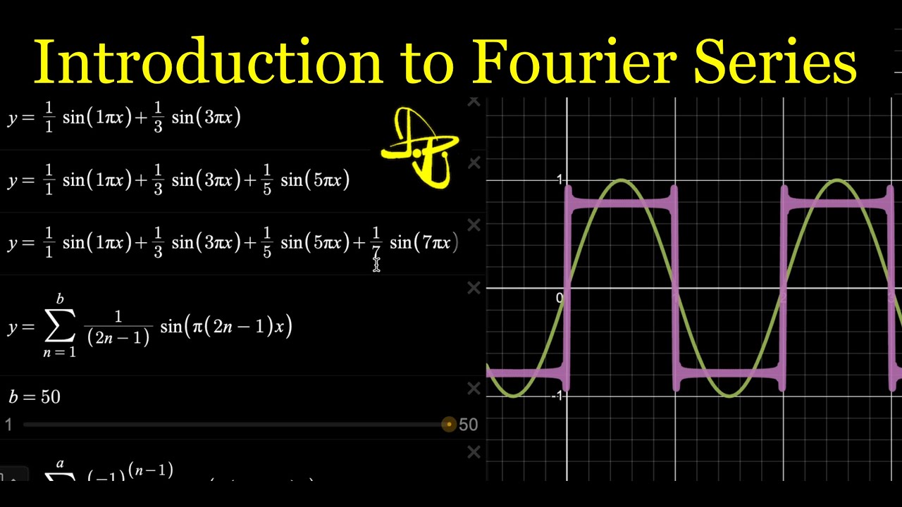
• 🔢 The concept of infinite sums is introduced to explain how a sum of waves can approximate a discontinuous function, such as a step function, through the limit of partial sums.
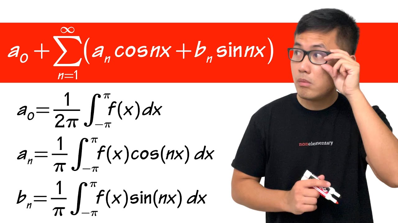
• 📉 The video delves into the technicalities of Fourier series, including the computation of coefficients for the series, which are found through integrals of the function.
• 🎨 The broader view of complex functions and rotating vectors is presented as a generalization of the real-valued functions typically used in Fourier series, providing a richer context for understanding the mathematics.

Q & A

What is a complex Fourier series?

A complex Fourier series is a mathematical technique used to decompose a function into a sum of rotating vectors, each with a constant integer frequency. It's a generalization of the more familiar Fourier series that deals with sine and cosine waves, allowing for a broader range of functions to be represented.

How does the animation with 300 rotating arrows relate to complex Fourier series?

The animation demonstrates the concept of complex Fourier series by showing how a complex shape can be drawn over time by adding together the motion of multiple arrows, each rotating at a constant frequency. This illustrates the idea of breaking down a function into simpler, oscillatory components.

What is the significance of being able to control the initial size and angle of each vector in a complex Fourier series?

Controlling the initial size and angle of each vector allows for the creation of a wide variety of shapes and patterns over time. This customization is essential for the practical application of Fourier series in various fields, as it enables the representation and manipulation of complex functions.

How does the concept of Fourier series relate to the heat equation?

Fourier series is intrinsically linked to the heat equation through the work of Joseph Fourier, who developed the series to solve the heat equation. The heat equation describes how temperature distributions evolve over time, and Fourier's method of breaking down functions into simpler components allowed for the equation's solutions to be found under various initial conditions.

What is the role of linearity in the context of the heat equation and Fourier series?

Linearity is crucial because it means that the sum of two solutions to the heat equation is also a solution, and solutions can be scaled by constants. This property allows for the construction of custom solutions by combining and scaling an infinite set of basic solutions, which are the exponentially decaying cosine waves in the context of Fourier series.

Why is the concept of infinite sums important in understanding Fourier series?

Infinite sums are important because they allow for the representation of functions that cannot be accurately represented by finite sums alone. In the context of Fourier series, infinite sums enable the approximation of non-periodic, discontinuous, or complex functions by combining an infinite number of simpler, periodic components.

How does the concept of complex numbers and complex exponentials contribute to the understanding of Fourier series?

Complex numbers and complex exponentials provide a powerful framework for understanding and computing Fourier series. They allow for the representation of rotating vectors and the generalization of Fourier series to functions with complex outputs, which simplifies computations and offers a deeper insight into the underlying mathematics.

What is the significance of the formula e^(i*t) in Fourier series?

The formula e^(i*t), representing a complex exponential, is fundamental in Fourier series because it describes a point moving around the unit circle in the complex plane as time 't' progresses. This property is used to model the rotating vectors that are the building blocks of the Fourier series decomposition.

How are the coefficients in a Fourier series calculated?

The coefficients in a Fourier series are calculated using integrals that essentially average the function over a period. For a function f(t), the coefficient c_n is found by integrating f(t) multiplied by the complex exponential e^(-i*n*2*pi*t) over the interval [0, 1], and then multiplying by the appropriate normalizing factor.

What is the practical application of Fourier series in solving differential equations?

Fourier series are used to solve differential equations by expressing complex functions as a sum of simpler, exponential functions. This allows for the application of linearity properties and the superposition principle, enabling the construction of solutions for a wide range of initial conditions and boundary conditions.

Outlines

00:00

🔍 Introduction to Complex Fourier Series

The paragraph introduces the concept of complex Fourier series through the lens of an animation featuring 300 rotating arrows. Each arrow rotates at a constant frequency, and their collective motion traces out intricate shapes over time. The speaker emphasizes the stark contrast between the simplicity of individual arrow movements and the resulting complex patterns they form when combined. The audience is encouraged to appreciate the beauty and complexity of the animation, which is a visual representation of the mathematical idea that simple components can create complex outcomes. The paragraph also sets the stage for a deeper exploration of Fourier series, hinting at their origins in solving the heat equation and their broader applications in various fields.

05:04

🌡️ Fourier Series and the Heat Equation

This paragraph delves into the historical context of Fourier series, explaining how they were developed as a solution to the heat equation. The heat equation describes how temperature distributions evolve over time, and Fourier's insight was to express any initial temperature distribution as a sum of sine waves. The paragraph discusses how certain boundary conditions lead to the use of cosine functions instead of sine waves and how these solutions can be combined to create custom solutions for different initial conditions. The speaker highlights the linear property of the heat equation, which allows for the addition of solutions and the scaling of them to fit specific scenarios. The paragraph also touches on the idea that the complexity of the heat distribution's evolution is captured by the different decay rates of the frequency components, leading to the concept of Fourier series as a way to describe and control complex phenomena through simple mathematical constructs.

10:05

🌟 The Immortality of Fourier's Legacy

The speaker reflects on the enduring impact of Fourier's work, noting that his ideas have become synonymous with the analysis of functions as combinations of simple oscillations. The paragraph explores the question of how to express non-wavy, discontinuous functions, like a step function, as sums of sine waves. It discusses the challenge of representing such functions using waves that satisfy specific boundary conditions and how Fourier's approach to using infinite sums of sine waves provides a solution. The concept of infinite sums is explained, drawing an analogy with the sum of rational numbers converging to an irrational number. The paragraph also raises philosophical questions about the nature of solving partial differential equations with discontinuous initial conditions and the completeness of Fourier series in representing all functions, hinting at deeper mathematical discussions.

15:10

🔄 Complex Numbers and Rotating Vectors in Fourier Series

The paragraph shifts the discussion to a more general view of Fourier series using complex numbers and rotating vectors. It explains how functions with real number outputs can be seen as one-dimensional pencil sketches, and how the decomposition into rotating vectors can be visualized. The speaker introduces the concept of complex exponentials, e to the i times t, which describes a point moving around the unit circle in the complex plane, and how this is fundamental to understanding Fourier series. The paragraph also discusses how the complex plane allows for a cleaner and more intuitive understanding of the computations involved in Fourier series, setting the stage for further exploration of related mathematical concepts like the Laplace transform and the importance of exponential functions.

20:11

📐 Computing Fourier Coefficients and Applications

This paragraph focuses on the practical computation of Fourier coefficients, which are essential for expressing a function as a sum of rotating vectors. The speaker describes how to find the constant term of a Fourier series by averaging the function over its input range, equating this to the calculation of an integral. The paragraph then explains how to compute the coefficients for non-constant terms by multiplying the function by a complex exponential that 'freezes' the corresponding rotating vector, allowing its coefficient to be isolated through averaging. The speaker also touches on the numerical methods used to compute these integrals and how the number of vectors used in the approximation affects the accuracy of the result. The paragraph concludes with a practical example of using Fourier series to model a step function, which has applications in understanding heat dissipation between two rods at different temperatures.

Keywords

💡Fourier Series

Fourier Series is a mathematical tool that decomposes functions into a sum of simple sine and cosine waves. In the context of the video, it's used to explain how complex patterns can be broken down into simpler components. The video script mentions that Fourier Series are not only limited to sine waves but can also be generalized to rotating vectors, which is a broader concept that includes the traditional sine wave decomposition as a special case.

💡Complex Numbers

Complex numbers are numbers that consist of a real part and an imaginary part, usually written as a + bi, where 'i' is the square root of -1. The video script uses complex numbers to represent rotating vectors in two dimensions, which simplifies the computation and visualization of Fourier Series. The concept is crucial as it allows for a more general treatment of functions, not just those with real number outputs.

💡Heat Equation

The heat equation is a partial differential equation that describes how the distribution of heat (or variation in temperature) evolves over time. In the video, the heat equation serves as the original motivation for the development of Fourier Series. The script explains how Fourier Series can be used to solve the heat equation for specific initial conditions, such as a rod with a temperature distribution that looks like a cosine wave.

💡Linear Equations

Linear equations are those that are linear in the unknown functions and their derivatives. The video script discusses the heat equation as a linear equation, which means solutions can be combined and scaled to construct new solutions. This property is essential for the application of Fourier Series, as it allows for the construction of solutions to the heat equation by combining simple cosine wave solutions.

💡Exponential Decay

Exponential decay refers to the decrease of a quantity at a rate proportional to its current value. In the video, the script describes how higher frequency components in the Fourier Series of a solution to the heat equation decay faster over time, leading to a smoothing effect as the high-frequency terms approach zero.

💡Discrete vs. Continuous

The video script contrasts discrete sums, which are finite, with continuous or infinite sums, which can approach a limit. The concept is important in understanding how Fourier Series can approximate functions. While a finite number of terms in a Fourier Series will never perfectly represent a discontinuous function like a step function, an infinite sum can get arbitrarily close to the desired shape.

💡Complex Exponentials

Complex exponentials, such as e^(i*t), are used in the video to describe rotating vectors in the complex plane. These are fundamental to the generalization of Fourier Series to complex functions and are essential for solving differential equations. The video script explains how complex exponentials can be thought of as a shorthand for describing rotation, but they also play a deeper role in mathematical analysis.

💡Coefficients

Coefficients in the context of Fourier Series are the constants that multiply each sine or cosine term in the series. The video script describes how these coefficients determine the initial size and angle of the rotating vectors that make up the Fourier Series representation of a function. The script also explains how these coefficients can be calculated using integrals over the function.

💡Numerical Integration

Numerical integration is a method for approximating the value of a definite integral using numerical techniques. In the video, numerical integration is mentioned as a way to compute the coefficients of the Fourier Series. The script describes how this is done by summing the product of the function values and the exponential terms over many small intervals.

💡SVG

SVG (Scalable Vector Graphics) is a file format for defining images in terms of mathematical curves. The video script mentions using SVG files to define the paths for the animations, which allows for the function mapping from time to points in space to be predefined. This is used in conjunction with Fourier Series to animate the complex functions.

Highlights

The animation is created using a complex Fourier series, where each vector rotates at a constant integer frequency.

By adjusting the initial size and angle of each vector, any shape can be drawn over time.

The animation consists of 300 rotating arrows, showcasing the intricacy of the motion.

The complexity of the animation arises from the simple rotation of individual arrows.

The animation demonstrates how a swarm of simple motions can create coordinated complexity.

Fourier series can describe and control the animation's complexity through mathematical tuning.

Fourier series originated from the heat equation, which describes temperature distribution over time.

The heat equation is a linear equation, allowing for the combination of solutions to create new solutions.

Fourier proposed expressing any initial distribution as a sum of sine waves, even discontinuous ones.

The Fourier series can be used to solve the heat equation for any initial condition.

The coefficients in the Fourier series are found by integrating the function over the input range.

The Fourier series is a sum of complex exponentials, which are more general than sine waves.

The complex plane allows for a cleaner understanding of Fourier series and their applications.

The constant term in the Fourier series is the average value of the function over the input range.

The coefficients for non-constant terms are found by multiplying the function by a phase shift and integrating.

The Fourier series can be used to approximate any function, with increasing accuracy as more terms are included.

The step function example demonstrates how Fourier series can model real-world phenomena like heat dissipation.

The Fourier series has far-reaching implications beyond its origins in physics, with applications in various fields.

Transcripts

Here, we look at the math behind an animation like this one,

what's known as a complex Fourier series.

Each little vector is rotating at some constant integer frequency,

and when you add them together, tip to tail, the final tip draws out some shape over time.

By tweaking the initial size and angle of each vector,

we can make it draw pretty much anything we want, and here you'll see how.

Before diving into it all, I want you to take

a moment to just linger on how striking this is.

This particular animation has 300 rotating arrows in total.

Go full screen for this if you can, the intricacy is worth it.

Think about this, the action of each individual arrow is perhaps

the simplest thing you could imagine, rotation at a steady rate.

And yet the collection of all added together is anything but simple,

and the mind-boggling complexity is put into an even sharper focus the farther we

zoom in, revealing the contributions of the littlest, quickest,

and downright frenetic arrows.

When you consider the chaotic frenzy you're looking at,

and the clockwork rigidity underlying all the motions,

it's bizarre how the swarm acts with a kind of coordination to trace

out some very specific shape.

And unlike much of the emergent complexity you find elsewhere in nature,

this is something that we have the math to describe and to control completely.

Just by tuning the starting conditions, nothing more,

we can make this swarm conspire in all of the right ways to draw anything you want,

provided you have enough little arrows.

What's even crazier is that the ultimate formula for all of this is incredibly short.

Now often, Fourier series are described in terms of something that looks a little

different, functions of real numbers being broken down as a sum of sine waves.

That turns out to be a special case of this more general rotating vector

phenomenon that we'll build up to, but it's where Fourier himself started,

and there's good reason for us to start the story there as well.

Technically, this is the third video in a sequence about the heat equation,

what Fourier was working on when he developed his big idea.

I would like to teach you about Fourier series in a way that doesn't depend on

you coming from those chapters, but if you have at least a high-level idea for

the problem from physics which originally motivated this piece of math,

it gives some indication for just how unexpectedly far-reaching Fourier series are.

All you need to know is that we had a certain equation which tells us

how the temperature distribution on a rod would evolve over time,

and incidentally it also describes many other phenomena unrelated to heat.

While it's hard to directly use this equation to figure out what will happen to an

arbitrary heat distribution, there's a simple solution if the initial function just

happens to look like a cosine wave, with the frequency tuned so that it's flat at each

end point.

Specifically, as you graph what happens over time,

these waves simply get scaled down exponentially,

with higher frequency waves having a faster exponential decay.

The heat equation happens to be what's known in the business as a linear equation,

meaning if you know two solutions and add them up, that sum is a new solution.

You can even scale them each by some constant,

which gives you some dials to turn to construct a custom function solving the equation.

This is a fairly straightforward property that you can verify for yourself,

but it's incredibly important.

It means we can take our infinite family of solutions,

these exponentially decaying cosine waves, scale a few of them by some

custom constants of our choosing, and combine them to get a solution for a new,

tailor-made initial condition, which is some combination of cosine waves.

One important thing I'd like you to notice is that when you combine these waves,

because the higher frequency ones decay faster,

the sum you construct will tend to smooth out over time,

as all the high frequency terms quickly go to zero,

leaving only the low frequency terms dominating.

So in a funny way, all of the complexity in the evolution of this heat

distribution which the heat equation implies is captured by this

difference in the decay rates for the different pure frequency components.

It's at this point that Fourier gains immortality.

I think most normal people at this stage would say, well,

I can solve the heat equation when the initial distribution just happens to look like

a wave, or a sum of waves, but what a shame it is that most real world distributions

don't at all look like that.

I mean, for example, let's say you brought together two rods

which were each at some uniform temperature, and you wanted

to know what happens immediately after they come into contact.

To make the number simple, let's say the temperature of the left rod is 1 degree,

and the right rod is negative 1 degree, and that the total length,

L, of the combined two rods is 1.

What this means is our initial temperature distribution is a step function,

which is so obviously different from a sine wave, or the sum of sine waves,

don't you think?

I mean, it's almost entirely flat, not wavy, and for god's sake it's even discontinuous!

And yet Fourier thought to ask a question which seems absurd.

How do you express this as a sum of sine waves?

Even more boldly, how do you express any initial distribution as a sum of sine waves?

And it's more constrained than just that!

You have to restrict yourself to adding waves which satisfy a certain boundary condition,

and as we saw last video, that means working with these cosine functions whose

frequencies are all some whole number multiple of a given base frequency.

And by the way, if you were working with some different boundary condition,

say that the endpoints have to stay fixed, you'd have a different set of waves at

your disposal to piece together, in this case replacing that cosine expression with

a sine.

It's strange how often progress in math looks more like

asking a new question rather than simply answering old ones.

Fourier really does have a kind of immortality now,

with his name essentially synonymous with the idea of breaking

down functions and patterns as combinations of simple oscillations.

It's really hard to overstate just how important and far-reaching that idea

turned out to be, well beyond anything Fourier himself could have imagined.

And yet, the origin of all this is a piece of physics which,

at first glance, has nothing to do with frequencies and oscillations.

If nothing else, this should give you a hint about

the general applicability of Fourier series.

Now hang on, I hear some of you saying, none of these sums of sine waves that

you're showing are actually the step function, they're all just approximations.

And it's true, any finite sum of sine waves will never be perfectly flat,

except for a constant function, nor will it be discontinuous.

But Fourier thought more broadly, considering infinite sums.

In the case of our step function, it turns out to be equal to this infinite sum,

where the coefficients are 1, negative one third, plus one fifth, minus one seventh,

and so on for all the odd frequencies, and all of it is rescaled by 4 divided by pi.

I'll explain where those numbers come from in a moment.

Before that, it's worth being clear about what we mean by a phrase like infinite sum,

which runs the risk of being a little vague.

Consider the simpler context of numbers, where you could say,

for example, that this infinite sum of fractions equals pi divided by 4.

As you keep adding the terms one by one, at all times what you have is rational,

it never actually equals the irrational pi divided by 4.

But this sequence of partial sums approaches pi over 4, which is to say,

the numbers you see, while never equaling pi over 4,

get arbitrarily close to that value, and they stay arbitrarily close to that value.

That's all a mouthful to say, so instead we abbreviate

and just say the infinite sum equals pi over 4.

With functions, you're doing the same thing, but with many different values in parallel.

Consider a specific input, and the value of all

of these scaled cosine functions for that input.

If that input is less than 0.5, as you add more and more terms, the sum will approach 1.

If that input is greater than 0.5, as you add more and more terms,

it would approach negative 1.

At the input 0.5 itself, all of the cosines are 0,

so the limit of the partial sums is also 0.

That means that, somewhat awkwardly, for this infinite sum to be strictly true,

we have to prescribe the value of this set function at the point of

discontinuity to be 0, sort of halfway along the jump.

Analogous to an infinite sum of rational numbers being irrational,

the infinite sum of wavy continuous functions can equal a discontinuous flat function.

Getting limits into the game allows for qualitative changes,

which finite sums alone never could.

There are multiple technical nuances that I'm sweeping under the rug here.

Does the fact that we're forced into a certain value for the step function

at the point of discontinuity make any difference for the heat flow problem?

For that matter, what does it really mean to solve

a PDE with a discontinuous initial condition?

Can we be sure that the limit of solutions to the heat equation is also a solution?

And can we be sure that all functions actually have a Fourier series like this?

If not, when not?

These are exactly the kind of questions which real analysis is built to answer,

but it falls a bit deeper in the weeds than I'd like to go here,

so I'll relegate that all to links in the video's description.

The upshot is that when you take the heat equation solutions associated with

these cosine waves and add them all up, all infinitely many of them,

you do get an exact solution describing how the step function will evolve over time,

and if you had done this in 1822, you would have become immortal for doing so.

The key challenge in all of this, of course, is to find these coefficients.

So far, we've been thinking about functions with real number outputs,

but for the computations, I'd like to show you something more general than what

Fourier originally did, applying to functions whose output can be any complex number

in the 2D plane, which is where all these rotating vectors from the opening come

back into play.

Why the added complexity?

Well, aside from being more general, in my view, the computations become cleaner,

and it's easier to understand why they actually work.

More importantly, it sets a good foundation for the ideas that will come up later on

in the series, like the Laplace transform, and the importance of exponential functions.

We'll still think of functions whose input is some real number on a finite interval,

say from 0 up to 1 for simplicity, but whereas something like a temperature

function will have outputs on the real number line,

this broader view will let the outputs wander anywhere in the 2D complex plane.

You might think of such a function as a drawing,

with a pencil tip tracing out different points in the complex plane as the

input ranges from 0 to 1.

And instead of sine waves being the fundamental building block,

as you saw at the start, we'll focus on breaking these functions down

as a sum of little vectors, all rotating at some constant integer frequency.

Functions with real number outputs are essentially really boring drawings,

a one-dimensional pencil sketch.

You might not be used to thinking of them like this,

since usually we visualize such a function with a graph,

but right now the path being drawn is only in the output space.

If you do one of these decompositions into rotating vectors for a boring one-dimensional

drawing, what will happen is that the vectors with frequency 1 and negative 1 will

have the same length, and they'll be horizontal reflections of each other.

When you just look at the sum of these two as they rotate,

that sum stays fixed on the real number line, and it oscillates like a sine wave.

If you haven't seen it before, this might be a really weird way to think about what a

sine wave is, since we're used to looking at its graph rather than the output alone

wandering on the real number line, but in the broader context of functions with complex

number outputs, this oscillation on the horizontal line is what a sine wave looks like.

Similarly, the pair of rotating vectors with frequencies 2 and negative 2 will

add another sine wave component, and so on, with the sine waves we were looking

for earlier now corresponding to pairs of vectors rotating in opposite directions.

So the context that Fourier originally studied,

breaking down real-valued functions into sine waves,

is a special case of the more general idea of 2D drawings and rotating vectors.

And at this point, maybe you don't trust me that widening our view to

complex functions makes things easier to understand, but bear with me,

it's really worth the added effort to see the fuller picture,

and I think you'll be pleased with how clean the actual computation is in

this broader context.

You may also wonder why, if we're going to bump things up into two dimensions,

we don't just talk about 2D vectors, what does the square root

of negative one have to do with anything?

Well, the heart and soul of Fourier series is the complex exponential, e to the i times t.

As the input t ticks forward with time, this value walks

around the unit circle at a rate of one unit per second.

In the next video you'll see a quick intuition for why exponentiating imaginary

numbers walks around circles like this from the perspective of differential equations.

And beyond that, as the series progresses, I hope to give you some

sense for why complex exponentials like this are actually very important.

In theory, you could describe all of the Fourier series stuff purely in terms of vectors,

and never breathe a word of i, the square root of negative one.

The formulas would become more convoluted, but beyond that,

leaving out the function e to the x would somehow no longer authentically

reflect why this idea turns out to be so useful for solving differential equations.

For right now, if you want, you can think of e to the i t as a

notational shorthand for describing rotating vectors,

but just keep in the back of your mind that it is more significant than mere shorthand.

You'll notice I'm being a little loose with language using the words vector and complex

numbers somewhat interchangeably, in large part because thinking of complex numbers

as little arrows makes the idea of adding a lot of them together easier to visualize.

Alright, armed with the function e to the i times t,

let's write down a formula for each of these rotating vectors we're working with.

For right now, think of each of them as starting

pointing one unit to the right at the number 1.

The easiest vector to describe is the constant one, which stays at the number 1,

never moving, or if you prefer, it's quote-unquote rotating just at a frequency of 0.

Then there will be the vector rotating one cycle every second,

which we write as e to the 2 pi i times t.

That 2 pi is there because as t goes from 0 to 1,

it needs to cover a distance of 2 pi along the circle.

Technically in what's being shown, it's actually one cycle every 10 seconds

so things aren't too dizzying, I'm slowing everything down by a factor of 10.

We also have a vector rotating at one cycle per second in the other direction,

e to the negative 2 pi i times t.

Similarly, the one going two rotations per second is e to the 2 times 2 pi i times t,

where that 2 times 2 pi in the exponent describes how much distance is covered in one

second.

And we go on like this over all integers, both positive and negative,

with a general formula of e to the n times 2 pi times i t.

Notice, this makes it more consistent to write that constant vector

as e to the 0 times 2 pi times i t, which feels like an awfully

complicated way to write the number 1, but at least it fits the pattern.

The control that we have, the set of knobs and dials we get to turn,

is the initial size and direction of each of these numbers.

The way we control that is by multiplying each one by some complex constant,

which I'll call c sub n.

For example, if we wanted the constant vector not to be at the number 1,

but to have a length of 0.5, c sub 0 would be 0.5.

If we wanted the vector rotating at 1 cycle per second to start off at an

angle of 45 degrees, we'd multiply it by a complex number which has the effect

of rotating it by that much, which you can write as e to the pi fourths times i.

And if its initial length needed to be 0.3, then the

coefficient c sub 1 would be 0.3 times that amount.

Likewise, everyone in our infinite family of rotating vectors has some complex constant

being multiplied into it, which determines its initial angle and its total magnitude.

Our goal is to express any arbitrary function f of t,

say this one that draws an eighth note as t goes from 0 to 1,

as a sum of terms like this, so we need some way of picking out these constants

one by one, given the data of the function itself.

The easiest of these to find is the constant term.

This term represents a sort of center of mass for the full drawing.

If you were to sample a bunch of evenly spaced values for the

input t as it ranges from 0 to 1, the average of all the outputs

of the function for those samples would be the constant term c0.

Or more accurately, as you consider finer and finer samples,

the average of the outputs for these samples approaches c0 in the limit.

What I'm describing, finer and finer sums of a function for samples of

t from the input range, is an integral, an integral of f of t from 0 to 1.

Normally, since I'm framing this all in terms of averages,

you would divide the integral by the length of the input range,

but that length is 1, so in this case, taking an integral and taking an

average are the same thing.

There's a very nice way to think about why this integral would pull out c0.

Remember, we want to think of this function as a sum of rotating vectors,

so consider this integral, this continuous average, as being applied to that whole sum.

The average of a sum like this is the same as the sum over the averages of each part.

You can read this move as a sort of subtle shift in perspective.

Rather than looking at the sum of all the vectors at each point in time

and taking the average value they sweep out, look at the average of an

individual vector as t goes from 0 to 1, and then add up all these averages.

But each of these vectors just makes a whole number of rotations around 0,

so its average value as t ranges from 0 to 1 will be 0.

The only exception is the constant term.

Since it stays static and doesn't rotate, its average value

is just whatever number it happened to start on, which is c0.

So doing this average over the whole function is a

sort of clever way to kill all the terms that aren't c0.

But here's the actual clever part.

Let's say you wanted to compute a different term, like c2,

sitting in front of the vector rotating two cycles per second.

The trick is to first multiply f of t by something that makes that vector hold still,

sort of the mathematical equivalent of giving a smartphone to an overactive child.

Specifically, if you multiply the whole function by e to the negative

2 times 2 pi i times t, think about what happens to each term.

Since multiplying exponentials results in adding what's in the exponent,

the frequency term in each of our exponents gets shifted down by 2.

So now, as we do our averages of each term, that c-1

vector spins around negative 3 times with an average of 0.

The c0 vector, previously constant, now rotates twice as t ranges from 0 to 1,

so its average is also 0.

And likewise, all vectors other than the c2 term make some whole number of rotations,

meaning they average out to be 0.

So taking the average of this modified function is

a clever way to kill all the terms other than c2.

And of course, there's nothing special about the number 2 here,

you could replace it with any other n, and you have a general formula for cn,

which is what we're looking for.

Out of context, this expression might look complicated, but remember,

you can read it as first modifying our function, our 2d drawing,

so as to make the nth little vector hold still,

and then performing an average which kills all the moving vectors and

leaves you only with the still part.

Isn't that crazy?

All of the complexity in these decompositions you're seeing of drawings into

sums of many rotating vectors is entirely captured in this little expression.

So when I'm rendering these animations, that's exactly what I'm having the computer do.

It treats the path like a complex function, and for a certain range of values n,

it computes this integral to find the coefficient c of n.

For those of you curious about where the data for a path itself comes from,

I'm going the easy route and just having the program read in an SVG,

which is a file format that defines the image in terms of mathematical curves rather

than with pixel values.

So the mapping f of t from a time parameter to points in space basically comes predefined.

In what's shown right now, I'm using 101 rotating vectors,

computing the values of n from negative 50 up to 50.

In practice, each of these integrals is computed numerically,

basically meaning it chops up the unit interval into many small pieces of size delta t,

and then adds up this value, f of t times e to the negative n 2 pi i t times delta t,

for each one of them.

There are fancier methods for more efficient numerical integration,

but this gives the basic idea.

And after you compute these 101 constants, each one determines an initial

angle and magnitude for the little vectors, and then you just set them all rotating,

adding them tip to tail as they go, and the path drawn out by the final

tip is some approximation of the original path you fed in.

As the number of vectors used approaches infinity,

the approximation path gets more and more accurate.

To bring this all back down to earth, consider the example we were looking at earlier,

of a step function, which remember was useful for modeling the heat dissipation

between two rods at different temperatures after they come into contact.

Like any real number valued function, the step function

is like a boring drawing that's confined to one dimension.

But this one is an especially dull drawing, since for inputs between 0 and 0.5,

the output just stays static at the number 1, and then it discontinuously

jumps to negative 1 for inputs between 0.5 and 1.

So in the Fourier series approximation, the vector sum stays really

close to 1 for the first half of the cycle, then quickly jumps to negative 1,

and stays close to that for the second half of the cycle.

And remember, each pair of vectors rotating in opposite directions

corresponds to one of the cosine waves we were looking at earlier.

To find the coefficients, you would need to compute this integral,

and for the ambitious viewers among you itching to work out some integrals by hand,

this is one where you can actually do the calculus to get an exact answer,

rather than just having a computer do it numerically for you.

I'll leave it as an exercise to work this out,

and to relate it back to the idea of cosine waves by pairing off the vectors

that rotate in opposite directions.

And for the even more ambitious, I'll leave another exercise up on the screen for

how to relate this more general computation with what you might see in a textbook

describing Fourier series only in terms of real valued functions with sines and cosines.

By the way, if you're looking for more Fourier series content,

I highly recommend the videos by Mathologer and The Coding Train,

and I'd also recommend this blog post, links of course in the description.

So on the one hand, this concludes our discussion of the heat equation,

which was a little window into the study of partial differential equations.

But on the other hand, this Fourier-to-Fourier series is a first glimpse at a deeper idea.

Exponential functions, including their generalization into complex

numbers and even matrices, play a very important role for differential equations,

especially when it comes to linear equations.

What you just saw, breaking down a function as a combination

of these exponentials and using that to solve a differential equation,

comes up again and again in different shapes and forms.

Thank you.