Samples from a Normal Distribution | Statistics Tutorial #4 | MarinStatsLectures
Summary
TLDRThis video script explores the concept of sampling in statistics, aiming to understand how sample data can be used to make inferences about a larger population. It uses R software and a web visualization tool to demonstrate how samples drawn from a normal distribution with a known mean and standard deviation can vary in appearance. The script emphasizes the importance of understanding these variations to accurately generalize findings back to the population.
Takeaways
- 📊 **Understanding Sample Behavior**: The video emphasizes the importance of understanding how samples behave to make inferences about a population.
- 🔍 **Generalization from Samples**: It's crucial to learn how samples might differ from the population to generalize findings accurately.
- 📚 **Statistical Inference**: The process of making statements about a population using sample data is called statistical inference.
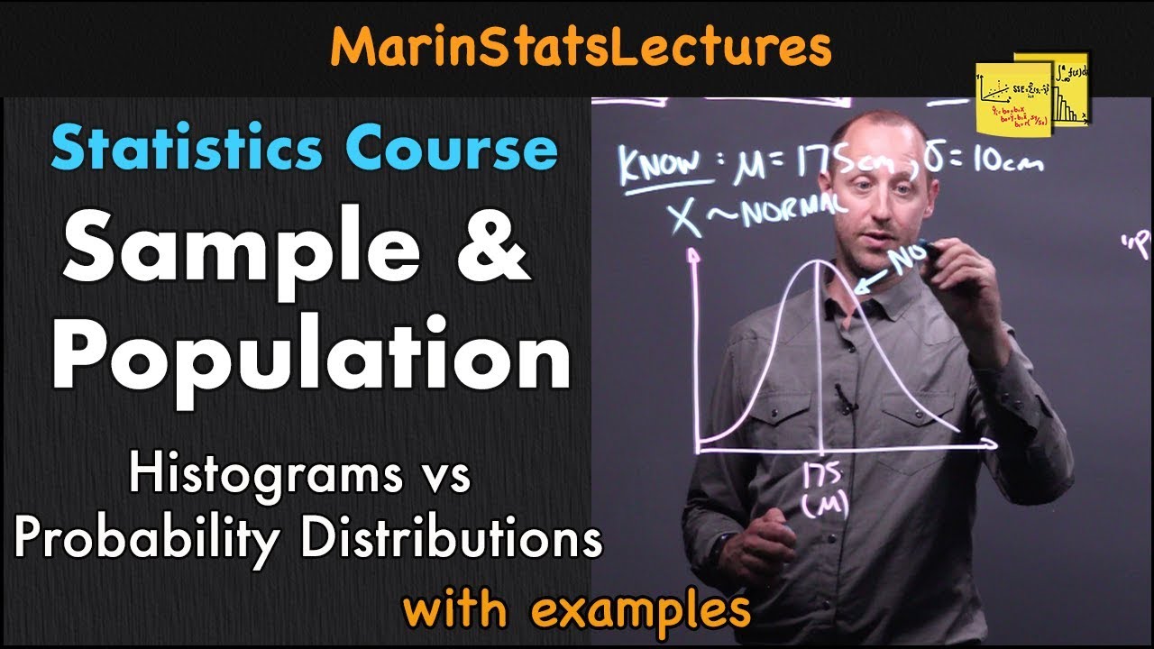
- 📈 **Normal Distribution Example**: The video uses a normal distribution with a mean of 150 and standard deviation of 40 as an example to illustrate sampling.
- 💻 **R Software Usage**: R software is used to simulate drawing samples and visualizing them through histograms.
- 📊 **Histograms for Visualization**: Histograms are generated to visualize the distribution of sample data.
- 🔢 **Sample Mean and Standard Deviation**: The video discusses calculating the sample mean and standard deviation to compare with the population parameters.
- 🔁 **Replicating Samples**: The process of taking multiple samples to observe variations is demonstrated.
- 🔄 **Increasing Sample Size**: The impact of increasing the sample size on the accuracy of sample statistics is explored.
- 🌐 **Web Visualization Tool**: A web tool is introduced for a more interactive way to visualize samples drawn from a population.
- 📝 **Practical Application**: The video encourages viewers to experiment with different sample sizes using R scripts and web tools for a deeper understanding.
Q & A
What is the main focus of the video?
-The video focuses on understanding how samples behave and how they can be used to make inferences about a population.
Why is it important to study sample behavior?
-Studying sample behavior is important because it helps in making accurate statements about a population using a sample, which is a subset of that population.
What statistical concept does the video use as an example?
-The video uses a normal distribution with a known mean of 150 and a standard deviation of 40 as an example to study sample behavior.
What software is used to simulate the sampling process in the video?
-The video uses R, a statistical software, to simulate the sampling process and generate histograms of the samples.
What is the significance of the sample size in the video?
-The video demonstrates that sample size can affect how closely a sample's statistics, like mean and standard deviation, approximate the true population values.
What is the sample size used in the initial simulation?
-The initial simulation uses a sample size of 20 observations drawn from the normal distribution.
How does the video demonstrate the variability of samples?
-The video demonstrates the variability of samples by repeatedly drawing samples of the same size and showing how the sample statistics can differ from one draw to another.
What is the concept of statistical inference mentioned in the video?
-Statistical inference is the process of making statements about a population based on the analysis of a sample drawn from that population.
Why might a sample not look normally distributed even if it comes from a normal population?
-A sample might not look normally distributed due to random sampling variability, especially when the sample size is small. This is known as sampling error.
What is the impact of increasing the sample size as shown in the video?
-Increasing the sample size tends to make the sample statistics, such as the mean and standard deviation, more closely resemble the true population values, leading to a more accurate representation of the population distribution.
What additional tool does the video suggest using to visualize samples?
-The video suggests using a web visualization tool as an alternative to R for visualizing samples and understanding their behavior.
What is the role of the mean and standard deviation in the context of this video?
-In the video, the mean and standard deviation of samples are used to estimate the corresponding population parameters and to illustrate how samples can vary in their representation of the population.
Outlines
📊 Understanding Sample Behavior
This paragraph introduces the concept of statistical inference, which involves using samples to make statements about a population. The narrator explains that while samples may not perfectly represent the population, understanding their behavior is crucial. As an example, the video demonstrates drawing samples from a normal distribution with a known mean of 150 and standard deviation of 40. The narrator uses R software to simulate this process, taking samples of size 20 and plotting histograms to visualize the distribution. Despite the samples not always appearing perfectly normal, the narrator emphasizes that they come from a population with a true mean and standard deviation. The sample means and standard deviations are calculated to show how they compare to the population values.
🔍 Exploring Sample Variation
The second paragraph continues the exploration of sample behavior by examining how sample estimates change with different sample sizes. The narrator uses R software to draw samples of size 50 and then 100, observing how the sample means and standard deviations approach the population values as the sample size increases. The video also uses a web visualization tool to demonstrate the same concept, showing that even with small sample sizes, the data is derived from a normally distributed population. The narrator encourages viewers to experiment with different sample sizes to gain a more intuitive understanding of sample variation and how it relates to the population parameters. The video concludes with a call to action for viewers to subscribe to the channel for more educational content.
Mindmap
Keywords
💡Sample
💡Population
💡Statistical Inference
💡Normal Distribution
💡Mean
💡Standard Deviation
💡Histogram
💡Sample Size
💡R (Statistical Software)
💡Web Visualization Tool
💡Simulation
Highlights
Importance of understanding sample behavior to generalize to a population
Statistical inference involves using samples to make statements about a population
Samples may not always perfectly represent the population
Example of drawing samples from a normal distribution with known mean and standard deviation
Using R software to simulate drawing samples and creating histograms
Observing sample mean and standard deviation may vary from the population values
First sample of 20 observations from the normal distribution
Sample mean of 146.66 and standard deviation of 34.96 from the first sample
Taking additional samples to observe variation
Second sample showing a sample mean of 163.6 and standard deviation of 39.7
Third sample with a sample mean of 149 and standard deviation of 40
Increasing sample size to 50 to see if estimates become more accurate
Sample of size 50 with a sample mean of 157 and standard deviation of 43
Observing that larger sample sizes may yield histograms that look more normal
Using a web visualization tool to draw samples and compare to the population
Web tool shows a sample of 100 observations from the normal distribution
Encouragement to experiment with different sample sizes to gain intuitive understanding
Availability of R script and web visualization link in the video description
Transcripts
In this video we're going to learn a little bit about how samples behave.
We need to learn a little bit about how samples behave in order to be able to
take a sample and generalize back to a population.
In statistical analysis, we will use a sample to try and make statements about a population but the
sample that we get won't always look exactly like the population, so we need
to learn a bit about how different might it look so that we can incorporate this
into our procedure for making statements about a population which we call
statistical inference; as an example let's consider drawing samples from a
normal distribution that has a mean of 150 and a standard deviation of 40,
Here we're looking at a population where we know the exact mean, standard
deviation and shape of the distribution; first we're going to look at doing this
using R (Software) and running some simulations and then we're going to look at it using a
web visualization tool. First I'm going to have R make a plot of this normal distribution
so we can see this is the true or theoretical distribution that
we're going to draw samples from. I'm going to start by taking a sample of 20
out of this population so we're gonna let R (Statistical Software) know we'd like to take a sample of
size 20, here I'm going to ask R to draw a sample from a normal distribution
of size 20 and the normal has a mean of 150 a standard deviation of 40; and then
I'm going to ask R to give us a histogram of these 20 observations. Now
taking a look at this here you might be tempted to say this data does not look
normally distributed but because we're in a kind of artificial simulation
environment here we know that these 20 observations came from a population that
was perfectly normally distributed with a mean of 150, standard deviation of 40
let's also take the mean of our sample here we can see it came out to be 146.66
and again we know at the population these individuals were drawn
from a population that has a true mean of 150; let's take a look at our sample
standard deviation came out to be 34.96 and again we know that at
the population level these 20 individuals came from a population that
has a standard deviation of 40. So this gave us an a little bit of an idea of
how our sample varied from the true values; let's just take a look at doing
that again. To do so I'm just going to re-submit this code asking R to take
another sample of 20 from this population. We can see the histogram here
again this came from a population that is normally distributed we can see a
sample mean of 163.6, sample standard deviation of 39.7
Let's ask R to do this again. Again looking at this histogram well it
may not look or you may not want to say that this looks normally distributed we
know that it came from a normal distribution sample mean of 149 sample
standard deviation of 40. Let's ask R to draw another sample of 20 again this
data came from a normal that one actually looks a little bit more like
what we might call normal let's ask R for one more again this data came from a
normal distribution we can think of what happens if we increase the sample size
so let's ask R to draw samples of size 50 from this population so I've
increased n up to 50 and now I'm going to ask R to draw a sample of 50 from
this population make a histogram calculate the sample mean and sample
standard deviation; again these 50 observations came from a normal
distribution we know that sample mean of 157 sample standard deviation of 43
let's look at doing this a few more times grab another sample of 50 take a
look at the histogram sample mean and sample standard deviation let's do that
one more time again this data came from a normal distribution and one more so
again people might be the first time taking an intro stats course or I guess
less trained eye might look at a histogram like this and be tempted to say that it
looks skewed to the left or negatively skewed where in fact we know that this
data came from a normal distribution: a perfectly bell-shaped and symmetric
population so I'll leave this with you you can take this R-script and you can
try playing around with different sample sizes increase it to 100, 200 whatever
you like and see how the sample estimates change.
Now let's take a quick look at the same sort of example using a web visualization so using a slightly
nicer looking version or different looking version of the same exercise.
Here we can see we have this set up to draw samples of size 20 from a
population that has a mean of 150 standard deviation of 40 and if we ask
to show the population we can see that at the population level the distribution
is perfectly bell-shaped and symmetric or normal! okay I'm going to hide that
now let's ask it to draw a sample of 20 for us and we can see taking a look at
the histogram here while you may or may not be tempted to call this normally
distributed we know that it came from a normally distributed population let's
take a look at doing that again so I'm going to get another sample of 20
observations again this data here came from a normally distributed population
now you can play around with it if you want you can try increasing the sample
size seeing how the sample estimates vary. Let's quickly let's go up to a
large sample let's take 100 and see what it looks like here's our sample
of 100 observations this one doesn't look too bad but either way
we're in this kind of simulation world where we know at the population level
this data is normally distributed let's take a look at drawing one more sample
of 100; well that one looks pretty good so over the course we're going to
formalize these ideas a bit more mathematically we're going to get a more
exact understanding of how samples vary from the true or population value in the
mean time you can play around with these for the moment to get a bit more
intuitive understanding of how samples vary you can find the R script that I've
used in this video as well as a link to this web visualization in the video
description below. Make Sure to Subscribe to Marinstatlectures!
Посмотреть больше похожих видео
Sampling Distributions: Introduction to the Concept
Sample and Population in Statistics | Statistics Tutorial | MarinStatsLectures
Central Limit Theorem & Sampling Distribution Concepts | Statistics Tutorial | MarinStatsLectures
KUPAS TUNTAS: Apakah Perbedaan Statistik Inferensial dengan Statistik Deskriptif ?
Normal Distribution, Z-Scores & Empirical Rule | Statistics Tutorial #3 | MarinStatsLectures
Population vs Sample
5.0 / 5 (0 votes)