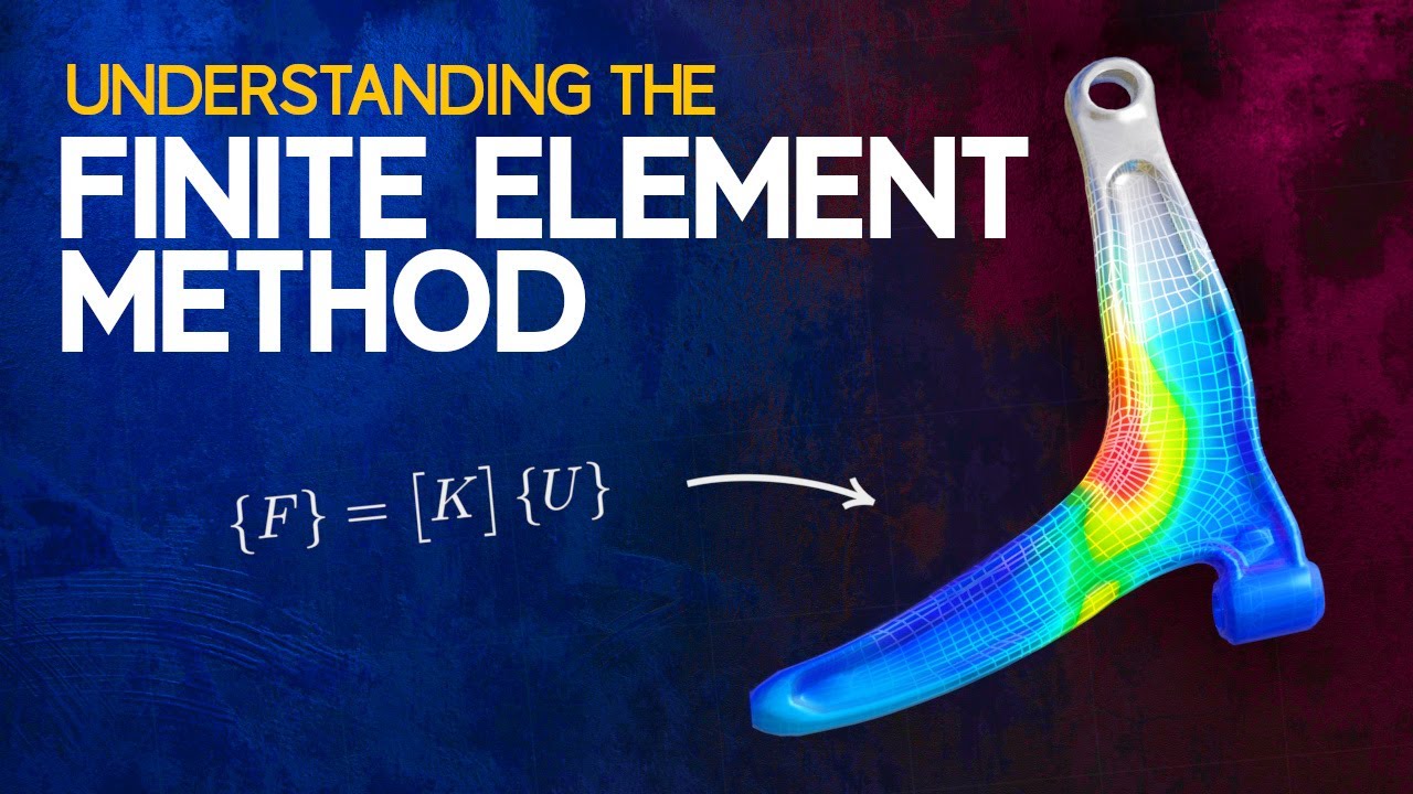
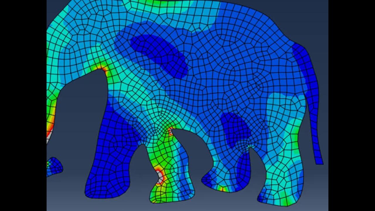
FEA 26: Isoparametric Elements

Summary

This video explains isoparametric elements, a type of finite element used in structural analysis, where transformations occur between local (natural) and global coordinate systems. Isoparametric elements employ the same shape functions for both displacement interpolation and coordinate mapping. The video covers the benefits of mapping four-sided and 3D elements from natural coordinates to global coordinates, and explores the process of creating stiffness matrices through this mapping. Additionally, it explains the importance of the Jacobian matrix in ensuring accurate integration and evaluating element quality.

Takeaways

• 🔄 Isoparametric elements use the same shape functions to interpolate displacement and map between local and global coordinate systems.
• 🌍 Elements can be defined either directly in the global system or transformed from a local system, with isoparametric elements opting for the latter.
• 🟥 Defining four-sided elements directly in global coordinates can be complex due to shape variations, whereas using local coordinates simplifies element definitions.
• 📐 The local coordinate system for isoparametric elements is called 'natural coordinates,' often using variables like 's' and 't'.
• 🔗 A key aspect of isoparametric elements is mapping from the natural coordinate system to the global coordinate system.
• 📊 The mapping between natural and global coordinates uses shape functions that are typically employed to interpolate displacements.
• 🧮 Calculating element stiffness matrices becomes easier using this mapping, reducing complex global integrations into simple operations in the natural coordinate system.
• 🔍 The Jacobian matrix plays a crucial role in the transformation, linking global and natural coordinates and helping with derivative calculations.
• 💡 The determinant of the Jacobian matrix represents the ratio of the element's area in global and natural coordinates, providing insight into element quality.
• ⚠️ A well-formed element has a nearly constant Jacobian, and a good rule of thumb is that the minimum determinant should be at least 70% of the maximum.

Q & A

What are isoparametric elements?

Isoparametric elements are a type of finite element where the same shape functions are used to interpolate both displacements and map from a local coordinate system (natural coordinates) to a global coordinate system.

What is the advantage of using a local coordinate system in isoparametric elements?

Using a local coordinate system simplifies element definitions because a single mathematical mapping can be applied to all elements, regardless of their shape or orientation in the global coordinate system. This makes the process of defining elements more consistent and easier.

Why is transformation necessary for four-sided elements in a mesh?

Four-sided elements in a mesh can take on a variety of shapes and orientations. Defining each one directly in the global coordinate system would be complex and inefficient, so a local-to-global transformation simplifies this process and ensures consistency across the mesh.

What are natural coordinates in the context of isoparametric elements?

Natural coordinates refer to a fixed coordinate system (often labeled s and t) used to define the element within a standard shape, such as a square. These coordinates are used in the local system for transformation to the global coordinate system.

How does mapping from natural coordinates to global coordinates work in isoparametric elements?

Mapping is achieved by using the shape functions that define the displacement in the local coordinate system to relate the positions in the natural (local) coordinate system to the global coordinates. This ensures a consistent mapping for all elements.

What role do shape functions play in isoparametric elements?

Shape functions in isoparametric elements are used for two purposes: they interpolate displacement within the element, and they are used to map the positions from the natural (local) coordinate system to the global coordinate system.

How is the stiffness matrix computed in isoparametric elements?

The stiffness matrix is computed by integrating over the element, but rather than integrating in global coordinates (which would be complex), the integration is performed in the natural coordinate system (with limits from -1 to 1), making the process easier and more consistent.

What is the Jacobian matrix, and why is it important in the mapping process?

The Jacobian matrix represents the derivatives of global coordinates with respect to natural coordinates. It captures the transformation information needed to map between the two coordinate systems. The inverse of the Jacobian is used to calculate derivatives needed for strain and stiffness matrix calculations.

Why is the determinant of the Jacobian matrix important?

The determinant of the Jacobian matrix represents a scale factor that is the ratio of the element's area in the global coordinates to the area in the natural coordinates. This scale factor is critical for accurate integration and stiffness matrix calculation.

What does it mean if the determinant of the Jacobian matrix is not constant?

If the determinant of the Jacobian matrix is not constant, it indicates that the element is not well-shaped or uniform. This could lead to an approximation error during numerical integration, affecting the accuracy of the stiffness matrix and the overall element quality.

Outlines

00:00

🔍 Introduction to Isoparametric Elements

This paragraph introduces isoparametric elements, which involve defining an element in a local coordinate system and transforming it to a global one. Unlike regular elements, isoparametric elements use the same shape functions for displacement interpolation and for mapping between local and global systems. The discussion begins with comparing element transformation options, emphasizing the challenges of defining elements directly in a global coordinate system, especially for non-square four-sided figures. Using a local coordinate system simplifies this, despite the complexity of the transformation.

05:00

🔄 Mapping Between Coordinate Systems

The focus here is on the transformation process between the natural coordinate system (local) and the global coordinate system for isoparametric elements. A square element in the natural system is mapped onto a more complex shape in the global system, with nodes being transformed accordingly. This mapping uses shape functions to relate coordinates in both systems. The main challenge is ensuring that the transformation remains consistent across all elements. The same shape functions used for displacement are now employed to map positions between these two coordinate systems.

10:01

📐 Understanding the Matrix Mapping

This section explains how the position within the element (in terms of x and y coordinates) is derived using shape functions and a vector of nodal positions in the global system. The shape function matrix used for displacement is now applied to nodal positions, creating a mapping system. This transformation results in a one-to-one correspondence between points in the local and global systems, simplifying complex calculations like stiffness matrix integration by transforming operations into the natural coordinate system.

15:01

📊 Chain Rule and Jacobian Matrix Derivation

The discussion moves into how the Jacobian matrix is derived through the chain rule to calculate the necessary derivatives of shape functions with respect to global coordinates. The Jacobian matrix, which consists of partial derivatives of global coordinates with respect to natural coordinates, plays a critical role in transforming these derivatives. The inverse of this matrix is used to find derivatives of shape functions, aiding in mapping and integration in finite element analysis (FEA). This matrix allows the transformation of operations from global to local systems in a manageable way.

Keywords

💡Isoparametric Elements

Isoparametric elements are a type of finite element where the same shape functions used to interpolate displacements are used to map from a local coordinate system (natural coordinates) to a global coordinate system. This technique simplifies the transformation process, making it easier to handle elements of complex shapes within finite element analysis. In the video, the term is introduced as the main topic, focusing on how this element type is essential for transforming local system coordinates to global ones.

💡Local Coordinate System

The local coordinate system is the reference framework where the properties of finite elements are initially defined before being transformed into a global coordinate system. In the context of isoparametric elements, the local system helps standardize the geometry, allowing elements to be mapped easily. The video mentions that using a local coordinate system is crucial to simplify complex mesh configurations in finite element analysis.

💡Global Coordinate System

The global coordinate system is the overall coordinate system used to define the positions of elements in the larger structure or model. The transformation from the local to global system allows for more uniform handling of elements across different configurations. The video discusses how defining elements directly in the global system can be tedious, especially for irregular shapes, making transformation from local coordinates a more efficient approach.

💡Shape Functions

Shape functions are mathematical expressions used to interpolate displacement, strains, and stresses within an element. In isoparametric elements, the same shape functions are used to map positions between the local and global coordinate systems, as well as to interpolate displacement. The video highlights how these functions are reused for both displacement calculations and the mapping process, making them central to isoparametric transformations.

💡Natural Coordinates

Natural coordinates (often denoted as S and T) refer to the local coordinate system used in isoparametric elements to standardize the size and shape of the element. This system allows for simpler interpolation of element properties. In the video, the term is introduced as a replacement for the local coordinate system when discussing isoparametric elements, emphasizing how it enables uniform definitions for elements despite their actual shape in global coordinates.

💡Mapping

Mapping is the process of converting an element's position from the natural (local) coordinate system to the global coordinate system. In isoparametric elements, this transformation is done using shape functions. The video describes the mapping process as essential for handling elements of different shapes and orientations within finite element analysis, ensuring consistency across different configurations.

💡Jacobian Matrix

The Jacobian matrix is used in the transformation process between natural and global coordinates. It contains the derivatives of global coordinates with respect to natural coordinates, encapsulating the geometric mapping of the element. The video introduces the Jacobian as the key matrix that allows for the calculation of derivatives, essential for strain and stiffness computations in finite element analysis.

💡Stiffness Matrix

The stiffness matrix is a fundamental component of finite element analysis, representing the relationship between nodal displacements and applied forces. In the context of isoparametric elements, it is computed using shape functions and the Jacobian matrix, which simplifies integration over complex element shapes. The video explains how transforming to natural coordinates makes this integration process more efficient, as it avoids calculating over irregular shapes in the global system.

💡Bilinear Quadrilateral Element

A bilinear quadrilateral element is a type of finite element with four nodes, where the displacement field is approximated by bilinear shape functions. The video uses this element as an example to explain how natural coordinates and shape functions work in isoparametric mapping. It shows how a standard-sized bilinear element in natural coordinates can be transformed into different shapes in global coordinates while maintaining consistency in calculations.

💡Chain Rule

The chain rule is a mathematical principle used to calculate the derivative of a function with respect to one variable when it depends on other variables. In the context of isoparametric elements, the chain rule helps in finding the derivatives of shape functions with respect to global coordinates by first taking derivatives with respect to natural coordinates. The video explains how the chain rule is applied to derive the necessary transformations for strain and displacement computations.

Highlights

Introduction to isoparametric elements and their importance in transforming between local and global coordinate systems.

Isoparametric elements use the same shape functions to interpolate displacements and to map from local to global coordinates.

Defining elements directly in the global system can be complex, especially for four-sided figures, making local system transformation preferable.

Natural coordinates are used in the local system for isoparametric elements, typically labeled as S and T, to simplify element definitions.

A key advantage of the local-to-global transformation is reducing the complexity of handling different element shapes.

The transformation challenge is to relate the local system's basic square element to the global system’s irregularly shaped element.

Shape functions, used to define displacement interpolation, are also employed to map positions from natural to global coordinates.

The mapping matrix for position interpolation reuses the same shape function matrix used for displacements, allowing consistency across the element.

The Jacobian matrix is used to define the transformation between natural and global coordinates, critical for calculating element stiffness.

The inverse of the Jacobian matrix allows calculating the partial derivatives of shape functions with respect to global coordinates.

Chain rule derivatives are used to connect shape function derivatives in the natural coordinate system to global coordinates.

The determinant of the Jacobian matrix serves as a scale factor, representing the ratio of the element area in global versus natural coordinates.

A constant Jacobian determinant indicates high-quality elements, while variations imply numerical integration approximations during stiffness calculations.

When the Jacobian determinant is not constant, the element quality can be assessed by comparing the minimum to maximum determinant ratios.

A rule of thumb is that the minimum determinant should be at least 70% of the maximum to ensure good element quality.

Transcripts

this video introduces isoparametric

elements isoparametric elements are an

element type where we define the element

in a local coordinate system and then we

transform it to a global coordinate

system we've done that before with bar

and beam elements but now with

isoparametric it's a particular type of

transformation specifically if you look

at the term there ISO means same and

parametric is related to the parameters

that define our element so specifically

an isoparametric element is going to use

the same shape functions that are used

to interpolate displacement and we're

going to use those shape functions to do

a mapping from our local coordinate

system to our global coordinate system

before we get into isoparametric

elements let's quickly review what our

options are for element transformation

what we have is elements that we need in

2d space and we have a global coordinate

system so one option we have is that we

define every single element directly in

the global system the benefit of that is

we don't need to worry about

transformation at all everything's done

with a global coordinate system however

every four-sided figure has a different

shape in the global coordinate system

well not every every square is Silla

square but we have a lot of non square

four-sided figures that show up in a

typical mesh and every single one of

those will need its own definition in

the global system we even have to get

new definitions for rotated squares

diamond shapes for example it can be

done this process of defining the

element properties directly the global

system can be done for three noted or

triangular elements and it works very

successfully for those but four-sided

has dramatic shape changes that require

a different definition for every new

type of shape that the four-sided figure

can form into so the alternative is to

define the elements in some sort of

local system and then transform them to

the global system in order to do the

calculations that is by far easier even

though the transformation as you're

going to see gets a little bit messy

it's far easier because we have one

definition for every four-sided figure

then

so we get that simple single simple

definition but we have a transformation

challenge so we're going to have to

define some sort of mathematical mapping

between our local system and our global

system that is how most four-sided

figures are our maps are transformed

we're also going to see that for most

three-dimensional elements as well

you

before we get into how we map from a

local coordinate system to a global

let's focus in on that local coordinate

system for isoparametric elements

instead of talking about a local

coordinate system we call it the natural

coordinates for an element and here what

I've shown is the bilinear quadrilateral

element in its natural coordinate system

I'm going to call that coordinate system

SMT some other authors will use a

different set of variables here but it's

basically just not the global XY system

just like for the bilinear quadrilateral

we did previously the axes are centered

in the middle of the element but now the

element has a fixed size it is two units

tall and two units wide and the node

numbering is as shown so previously when

we looked at the bilinear quadrilateral

it had a width of two B and a height of

two H and here were the shape functions

for that element now what we're going to

do is convert that by setting B and H

equal to one so we have a standard size

and then we're going to take our s and

turn our X in turn into an S and our Y

in terms of T that gives us our new

shape functions defined in terms of the

natural coordinates s and T so now let's

talk about how we map from that natural

coordinate system over to our global XY

coordinate system so we start out in the

natural system with this basic square

element two by two dimensions and what

we want to do is map to a global system

where we have an element say that looks

like this where we have some nodes and

sines of corners but it's no longer a

square shape what we're trying to do is

relate these two shapes to each other so

that we can do things in the natural

coordinate system that's consistent

between every elements but the

properties will be relevant in the

global so here in the global system each

one of these nodes has nodes numbers x1

y1 x2 y2 and so on that each node there

we need to have some correspondence from

node 1 and global with coordinates of x1

y1

to node 1 in the natural with

coordinates of negative 1 negative 1 we

need to define a transformational

mapping that gives us the x coordinate

for every corresponding s and T

coordinate and similarly gives us the y

coordinate for every s and T coordinate

that means we can basically map on the

grid corresponding to the natural

coordinate system within this single

element that's fundamentally what we're

trying to do here put the S&T coordinate

system somewhat warped inside this

element when we do this mapping with

something called an isoparametric

element what we're going to use is the

elements shape functions previously

defined for displacements we're going to

use them to map the position from

natural to global so let's get started

on that mapping what I've got shown here

is the interpolation within the the

natural coordinate system of the

displacements so I have the N 1 n 2 & 3

and n 4 defined in terms of the natural

coordinates s and T and then I've got

you defined there as well so this we

know this definition that's how we find

displacement from degrees of freedom

it's the interpolation function so

displacement inside the element given by

the relationship between the nodal

displacements and the shape functions

what we want to do is now find the

positions inside an element in other

words x and y in terms of the nodal

positions so we're going to write a

relationship written in matrix form as

the vector X positions in the element is

equal to the shape function matrix

multiplied by a vector of nodal

positions rather than a vector of nodal

displacements so in other words this is

what we are writing as our mapping

system we're reusing those same shape

functions but now we're multiplying them

by the positions of each of the nodes in

the global system instead of multiplying

by them the

displacements of each of the notes so

that gives us the the full matrix form

is we have a vector of the nodal

positions x1 y1 into the position of

node 1 in global coordinates x2 y2 its

position of no.2 in global coordinates

and so on and then we have our shape

function matrix the exact same one we're

going to use for displacements but

remember it is now defined in terms of

the natural coordinate system s and T so

let's explore this mapping just a little

bit more we have what I'm calling a

little X vector that is the positions x

and y it's going to be equal to a shape

function matrix that's defined in terms

of the position in my natural coordinate

system and then I'm multiplying it by a

vector which is all of the nodal

positions in the global coordinates so

I'm mapping from the global over to the

local or vice versa it gives us a

one-to-one correspondence so there's one

point in the natural coordinate system

it will have a corresponding point in

the global system and the reason that

this helps us out is that we can define

our shape function matrix which we

already have in natural coordinates but

we can also define our B matrix that way

and we need to do some mapping we need

to take advantage of the mapping in

order to do that we'll see that in a

moment

secondly once we have the B matrix we

then need to calculate the stiffness

matrix to calculate the stiffness matrix

means integrating over the element every

element in global coordinates has a

different shape integrating over each of

those would be very complicated to try

to code but instead if we can use the

mapping to do our integration in the

natural coordinate system well that's

very easy we're going negative 1 to 1 in

X and y and then we're done so those are

the two real benefits we get out of

doing this mapping ok so let's work on

finding that V matrix it starts to get a

little bit hairy here so hang on tight

we know that V is going to be the

partial derivative matrix operator

multiplied by the shape function matrix

or in long form that looks like this but

we need to know the derivatives with

respect to X and Y because that's how

strain is related to displacement that's

where this came from the strain

displacement relationship however the

shape functions are now defined in terms

of our natural coordinate system so in

other words what we're looking for is

the derivative of say N 1 with respect

to X but N 1 is defined with respect to

s and T so what we're looking for are

the derivatives of the shape functions

with respect to x and y let's try the

chain rule for example DN I let's say I

is 1 2 3 or 4 plus DN I DX is going to

be equal to DN IDs times DSD X plus DN I

DT times DT DX that would be the chain

rule expansion of the derivative DN I DX

similarly for DN n IV Y we have a

similar relationship so that's the chain

rule expansion how does that help us

well see in just a moment let's write

this in matrix form because hey it's Fe

a and that's what we do so DN I DX DN i

dy becomes a vector and it's going to be

equal to a matrix which has the four

coefficients in there so d s DX DT DX D

s dy and DT dy notice that this is a

each one of these terms is a derivative

of the mapping the x2 T or y2 T of s DT

coordinate system that of course is all

going to be multiplied by my shape

function derivatives which I can now

solve for because shape functions are

defined directly in terms of s and T so

if we can figure out what's in that

matrix we can calculate the derivatives

of the shape functions with respect to x

and y which means we can then go and

find B but we know the vector with the

shape functions we don't know the

derivatives of the natural coordinates

with respect to the global remember our

mapping is X defined in terms of s and T

so we don't have the inverse let's

temporarily call that matrix that we

don't know

J and minus one the inverse of J so this

is the inverse of J why the inverse well

let me show you so J is something we

call the Jacobian matrix J inverse is

something we've just defined it's the

partial derivatives of s and T with

respect to x and y something that we

don't know on the other hand J is

something that we do know and I'll show

you how we get there so first off let's

take that expression and we'll multiply

both sides by the Jacobian J in other

words the inverse of the one we just saw

and when I do that I get DN d SD n DT is

equal to the Jacobian times DN DX and DN

D Y so now I have the thing that I don't

know on the right hand side multiplied

by something else that at the moment I

don't know and it's equal to the thing

that I do know not normally the

relationship that we'd like to use but

it's going to be helpful to us let's go

ahead and write out the chain rule

expansion of the two terms in the left

hand vector so DN DF is equal to DN DX

times DX DF plus DN D Y times dy DF

similarly we have a relationship like

that for DN DT a chain rule expansion

when I take that and I write it in

matrix form the left there vector looks

the same as what's above the matrix ends

up being each of those coefficients

again but now these are things that we

know D X D s and D Y D s are defined can

be directly calculated from our mapping

and then that's multiplied by again the

vector that we don't know but by

comparison of these two right-hand

equations we can see I've just defined

what the Jacobian is equal to it is four

terms which are the derivatives of my

global coordinates with respect to my

natural coordinates so you head hurting

yep

this actually works it makes sense it's

a little bit too a little bit difficult

to grasp so let's take it a step further

kind of bring it all home how do we get

to be with this information one of the

first things that we want to observe is

that if we can calculate J it's a 2 by 2

matrix we can find the inverse of it

once we calculate it so that's how we're

going to end up going back to that upper

left equation here which is going to

allow us to get those derivatives with

respect to x and y that we need to have

in the b matrix so now we have a

definition of a Jacobian matrix it is

the partial derivatives of global with

respect to local coordinates so the

matrix that we then need to find ni

derivative with respect to X and ni

derivative with respect to Y is the

inverse of that Jacobian and because

it's a 2 by 2 it has a simple definition

for the inverse so J inverse is defined

here we can use that to find each of

these partial derivative components of B

specifically what we're going to do is

for each of our shape functions 1 2 3 &

4 we're going to take the derivative

with respect to X or the derivative with

respect to Y that's what we're looking

for we don't know those they're going to

be equal to the Jacobian inverse

multiplied by the derivative of the

shape function with respect to s and T

the natural coordinate systems which

they are defined in terms of so there's

a lot more here that we're going to

explore in the next video just to wrap

this up I'm going to talk about a couple

of properties of this Jacobian matrix we

just created so first off note that its

terms are the derivatives of the global

coordinates with respect to the natural

coordinate system so it effectively is

that transformation matrix it's

capturing all the pertinent information

about our mathematical mapping another

interesting property is that when we

take the determinant of J that's a scale

factor it is actually equal to the ratio

of the elements area

global coordinates to the element area

in natural coordinates so ratio as in a

fraction we will use this property it'll

be critical when we find the stiffness

matrix for integration

another interesting point is that when

we have a high quality element that

determinant J is a constant term so when

we have an element which is a rectangle

J is constant

however if J is not constant in other

words it depends on position then the

numerical integration that we're going

to use to find the stiffness matrix is

not going to be exact it will be an

approximation that's going to be

important in the next video also if the

determinant is not constant we can use

the ratio of the maximum determinant

divided by the minim I'm sorry the

minimum divided by the maximum to assess

the degree of element quality and

specifically a good rule of thumb is

that the minimum should be at least 70%

of the maximum in other words it's close

to constant and then we can say we have

a good quality or a good shaped element