Graphing Trigonometric Functions
Summary
TLDRProfessor Dave's video script offers an in-depth exploration of trigonometric functions, focusing on domain and range, periodicity, and graphing techniques. He explains sine and cosine functions' domains as all real numbers and ranges from -1 to 1. Tangent's domain excludes points where cosine is zero, resulting in an undefined value. The script then delves into graphing transformations, such as amplitude adjustments, horizontal stretches, and phase shifts, using examples like 'Y = 4sin(2x - 2π/3)'. Lastly, it briefly covers the graphs of other trig functions like tangent, cotangent, secant, and cosecant, highlighting their unique characteristics and transformations.
Takeaways
- 📝 The domain of sine and cosine functions is all real numbers, as any angle can be input into these functions.
- 📝 The range of sine and cosine functions is from -1 to 1, inclusive, reflecting the y-values on the unit circle.
- 📝 Tangent function has a domain of all real numbers except where cosine is zero (i.e., not at π/2 + kπ where k is an integer), and its range is all real numbers due to its behavior as cosine approaches zero.
- 📝 Trigonometric functions are periodic with a period of 2π radians, meaning their values repeat every 2π radians.
- 📝 The graph of the sine function starts at 0, reaches 1 at π/2, and returns to 0 at π, then follows a similar pattern in the negative direction.
- 📝 Cosine function is similar to sine but starts at 1 and decreases to 0 at π/2, then to -1 at π, and repeats.
- 📝 Transformations such as amplitude changes, horizontal stretches or compressions, and phase shifts can be applied to trigonometric functions.
- 📝 The amplitude of a trigonometric function is determined by the absolute value of the coefficient in front of the sine or cosine function.
- 📝 The period of a trigonometric function is affected by the coefficient of the variable inside the function, being 2π divided by that coefficient.
- 📝 Vertical shifts move the graph up or down, while horizontal shifts (phase shifts) affect the starting point of the function, influenced by the coefficient of the variable.
- 📝 Other trigonometric functions like tangent, cotangent, secant, and cosecant have different graphs with asymptotes where the original functions had zeros.
Q & A
What are the domain and range of the sine function?
-The domain of the sine function is all real numbers, as it can accept any angle. The range is from negative one to one, inclusive, as the Y values on the unit circle fall within this interval.
How does the domain of the cosine function compare to that of the sine function?
-The domain of the cosine function is the same as that of the sine function, which is all real numbers, because it can also accept any angle.
Why is the range of the tangent function different from that of the sine and cosine functions?
-The range of the tangent function is all real numbers because as cosine approaches zero, the value of tangent (which is sine over cosine) approaches infinity.
What are the restrictions on the domain of the tangent function?
-The domain of the tangent function is almost all real numbers, but it cannot be evaluated when cosine is zero, which occurs at angles of half pi plus or minus multiples of pi.
What is the period of the sine and cosine functions?
-The period of the sine and cosine functions is two pi radians, as their values repeat every two pi radians.
How can you graph the sine function over one period?
-You start by plotting points on the Y-axis corresponding to the sine values at multiples of pi/6, then continue through the unit circle, noting the sine values decrease to zero at pi, become negative in the third quadrant, and return to zero at two pi.
What transformations can be applied to the sine function?
-Transformations include applying a coefficient to stretch or shrink the function (changing amplitude), a coefficient on X for horizontal stretch or compression (changing period), and vertical or horizontal shifts.
How does the amplitude of the sine function relate to the coefficient in front of it?
-The amplitude of the sine function is equal to the absolute value of the coefficient in front of it, such as in Y = A * sin(X).
What is the effect of a coefficient operating on X in the sine function?
-A coefficient operating on X in the sine function causes a horizontal stretch or compression, changing the period. For example, in Y = sin(B * X), the period is two pi over B.
How do vertical shifts affect the graph of the sine function?
-Vertical shifts add or subtract a constant from the sine function, moving the graph up or down without altering its shape. For instance, Y = sin(X) + 1 shifts the graph up by one unit.
What is the relationship between the graphs of the sine and cosine functions?
-The graphs of the sine and cosine functions are similar, with the cosine function being a phase shift of pi/2 to the right of the sine function.
Outlines

هذا القسم متوفر فقط للمشتركين. يرجى الترقية للوصول إلى هذه الميزة.
قم بالترقية الآنMindmap

هذا القسم متوفر فقط للمشتركين. يرجى الترقية للوصول إلى هذه الميزة.
قم بالترقية الآنKeywords

هذا القسم متوفر فقط للمشتركين. يرجى الترقية للوصول إلى هذه الميزة.
قم بالترقية الآنHighlights

هذا القسم متوفر فقط للمشتركين. يرجى الترقية للوصول إلى هذه الميزة.
قم بالترقية الآنTranscripts

هذا القسم متوفر فقط للمشتركين. يرجى الترقية للوصول إلى هذه الميزة.
قم بالترقية الآنتصفح المزيد من مقاطع الفيديو ذات الصلة
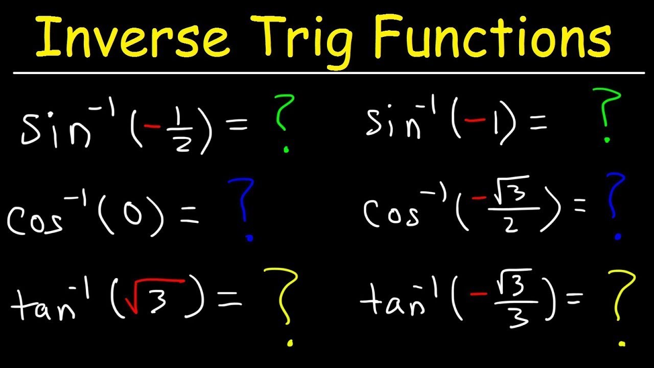
Evaluating Inverse Trigonometric Functions
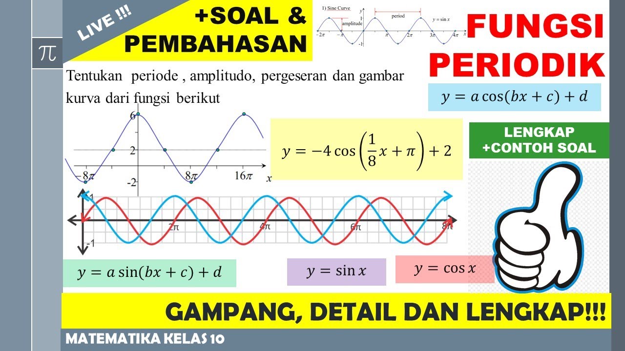
Fungsi 12: Fungsi Periodik dan Grafik Fungsi Trigonometri Kelas 10

Plus Two Maths Onam Exam | Continuity and Differentiability in 20 Min | Exam Winner Plus Two
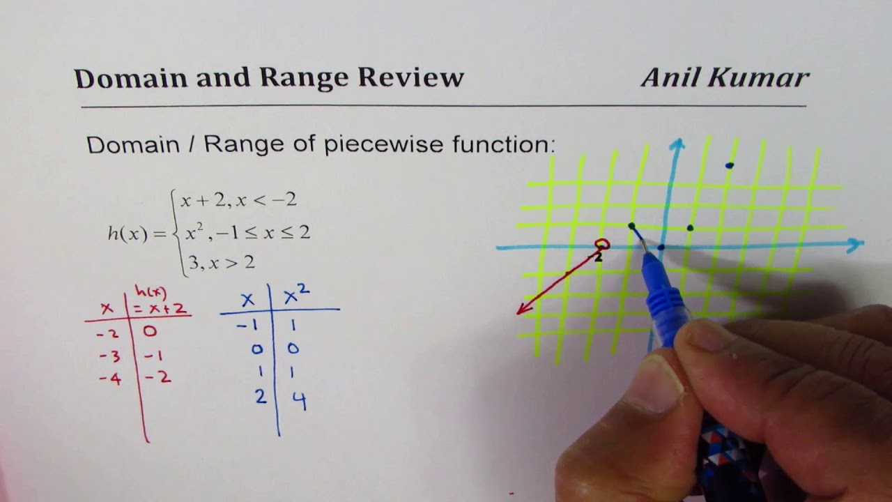
Piecewise Function Domain Range Quadratic Linear Constant

Back to Algebra: What are Functions?
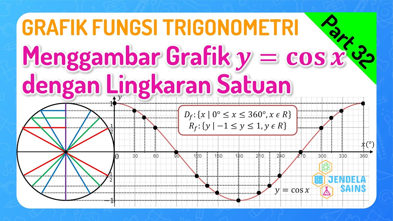
Trigonometri Matematika Kelas 10 • Part 32: Menggambar Grafik Fungsi y=cos x dengan Lingkaran Satuan
5.0 / 5 (0 votes)
