Training Neural Networks: Crash Course AI #4
Summary
TLDREn este episodio de Crash Course AI, Jabril nos introduce al concepto de redes neuronales artificiales, explicando cómo pueden aprender a resolver problemas al cometer errores y ajustar sus pesos mediante un algoritmo llamado retropropagación. Utiliza un ejemplo de predicción de la asistencia a una piscina basándose en datos como la temperatura y la humedad. A medida que se agregan más características, el proceso de optimización se vuelve más complejo, y aquí es donde las redes neuronales sobresalen. También se discuten temas como sobreajuste y la importancia de probar el sistema con nuevos datos.
Takeaways
- 🧠 Los cerebros artificiales pueden ser creados mediante redes neuronales, que consisten en millones de neuronas y billones de conexiones entre ellas.
- 🚀 Algunas redes neuronales son capaces de realizar tareas con mayor eficacia que los humanos, como jugar ajedrez o predecir el clima.
- 🔍 Las redes neuronales requieren de un proceso de aprendizaje a través de errores para resolver problemas, utilizando un algoritmo llamado retropropagación.
- 🏗️ Las redes neuronales se componen de dos partes principales: la arquitectura y las ponderaciones (weights), siendo estas últimas números que afinan el cálculo de las neuronas.
- 🔍 La optimización es la tarea de encontrar las mejores ponderaciones para una arquitectura de red neuronal, y se puede entender mejor con ejemplos prácticos.
- 📈 La regresión lineal es una estrategia de optimización utilizada por computadoras para encontrar una línea recta que mejor se ajuste a un conjunto de datos.
- 🌐 A medida que se consideran más características en los datos, la función de ajuste se vuelve más compleja y multidimensional, lo que es donde las redes neuronales son útiles.
- 🤖 El entrenamiento de una red neuronal implica ajustar las ponderaciones para minimizar el error y mejorar las predicciones en función de los datos de entrenamiento.
- 🔄 La retropropagación es un método esencial para que las redes neuronales aprendan, asignando la responsabilidad del error a las neuronas de capas anteriores y ajustando sus ponderaciones.
- 🌍 Al igual que los exploradores en un mapa, los algoritmos de aprendizaje deben navegar a través del espacio de soluciones para encontrar la combinación de ponderaciones que minimice el error.
- 🛡️ El sobreajuste es un riesgo en el aprendizaje de redes neuronales, donde el modelo se ajusta demasiado bien a los datos de entrenamiento y no generaliza bien a nuevos datos.
Q & A
¿Qué es una red neuronal y cómo se relaciona con el cerebro artificial?
-Una red neuronal es una estructura que imita la forma en que el cerebro humano procesa la información, compuesta por millones de neuronas y billones o trillones de conexiones entre ellas. Se utiliza en la creación de cerebros artificiales para realizar tareas complejas.
¿Por qué las redes neuronales necesitan aprender cometer errores?
-Las redes neuronales necesitan aprender cometer errores para ajustar sus pesos y arquitecturas de manera que mejoren su rendimiento en tareas específicas, similar al proceso de aprendizaje humano.
¿Qué es el backpropagation y cómo ayuda a las redes neuronales a aprender?
-El backpropagation es un algoritmo que permite a las redes neuronales distribuir la responsabilidad del error a través de las capas de la red, ajustando los pesos de las neuronas para reducir el error en futuras predicciones.
¿Cuáles son las dos partes principales de una red neuronal y qué función desempeñan?
-Las dos partes principales de una red neuronal son la arquitectura y los pesos. La arquitectura incluye las neuronas y sus conexiones, mientras que los pesos son números que afinan cómo las neuronas realizan sus cálculos matemáticos para obtener una salida.
¿Qué es la optimización en el contexto de las redes neuronales?
-La optimización en las redes neuronales se refiere al proceso de encontrar la mejor combinación de pesos para una dada arquitectura de red, con el objetivo de minimizar el error y mejorar la precisión de las predicciones.
¿Cómo se utiliza la regresión lineal para hacer predicciones en un ejemplo simple?
-La regresión lineal se utiliza para ajustar una línea recta a los datos de puntos en un gráfico, minimizando la suma de las distancias entre la línea y los puntos de datos para hacer predicciones basadas en características como la temperatura y el número de nadadores.
¿Qué significa 'línea de mejor ajuste' y cómo se relaciona con la regresión lineal?
-La 'línea de mejor ajuste' es el resultado de la regresión lineal que se ajusta lo más posible a los datos de entrenamiento, buscando minimizar el error y representar la relación entre las variables de forma más precisa.
¿Cómo se pueden mejorar los resultados de una red neuronal al considerar más características?
-Al incorporar más características, como la humedad o si está lloviendo, se pueden agregar dimensiones al modelo, lo que permite a la red neuronal aprender a resolver problemas más complejos y obtener resultados más precisos.
¿Qué es el peligro de sobreajuste en las redes neuronales y cómo se puede prevenir?
-El sobreajuste ocurre cuando una red neuronal se ajusta demasiado bien a los datos de entrenamiento, capturando relaciones espurios que no se aplican a nuevos datos. Se puede prevenir manteniendo la red neuronal lo suficientemente simple y evitando características irrelevantes.
¿Por qué es importante validar la capacidad de una red neuronal para responder a preguntas nuevas?
-Validar la capacidad de una red neuronal para responder a preguntas nuevas es crucial para asegurar que el modelo haya aprendido y no simplemente memorizado los datos de entrenamiento, lo que permitiría generalizar mejor en situaciones desconocidas.
Outlines

هذا القسم متوفر فقط للمشتركين. يرجى الترقية للوصول إلى هذه الميزة.
قم بالترقية الآنMindmap

هذا القسم متوفر فقط للمشتركين. يرجى الترقية للوصول إلى هذه الميزة.
قم بالترقية الآنKeywords

هذا القسم متوفر فقط للمشتركين. يرجى الترقية للوصول إلى هذه الميزة.
قم بالترقية الآنHighlights

هذا القسم متوفر فقط للمشتركين. يرجى الترقية للوصول إلى هذه الميزة.
قم بالترقية الآنTranscripts

هذا القسم متوفر فقط للمشتركين. يرجى الترقية للوصول إلى هذه الميزة.
قم بالترقية الآنتصفح المزيد من مقاطع الفيديو ذات الصلة

¿Qué es una Red Neuronal? Parte 3 : Backpropagation | DotCSV
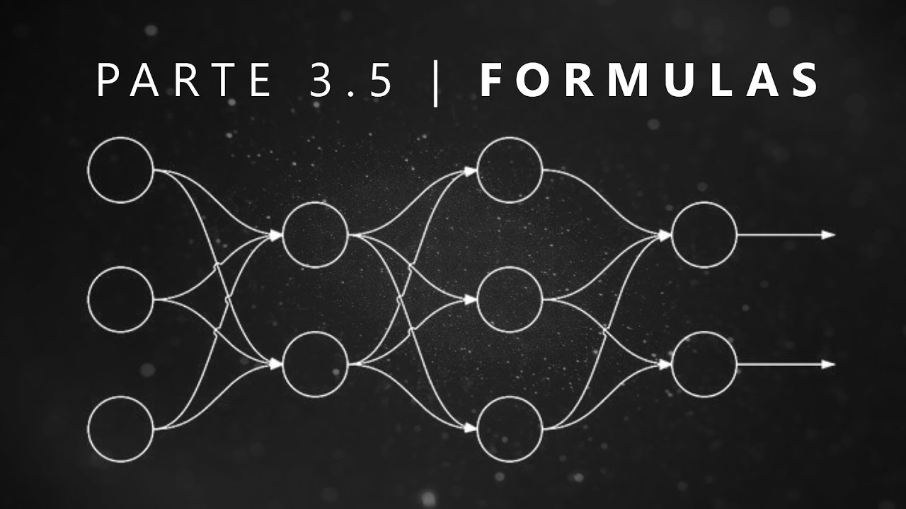
¿Qué es una Red Neuronal? Parte 3.5 : Las Matemáticas de Backpropagation | DotCSV
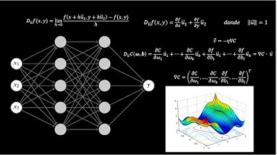
Las Matemáticas detrás de la IA

How Forward Propagation in Neural Networks works

¿Qué es una Red Neuronal? Parte 1 : La Neurona | DotCSV
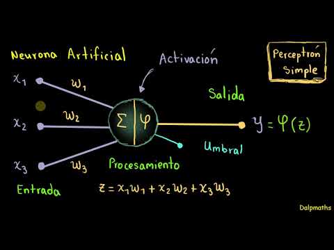
Redes neuronales: Introducción al perceptrón simple.
5.0 / 5 (0 votes)
