Aircraft simulation using MATLAB and Python
Summary
TLDRThis tutorial offers an in-depth look at longitudinal flight simulation using MATLAB and Python, focusing on the Convair 880 aircraft. It delves into estimating aerodynamic forces and coefficients, exploring the aircraft's longitudinal equations of motion, and solving them with both MATLAB and Python scripts. The study includes a steady-state condition and a disturbance scenario, showcasing the aircraft's response to a pitch rate disturbance. The tutorial provides access to the scripts and NASA's 1972 report on the Convair 880, offering a comprehensive guide for those interested in flight dynamics.
Takeaways
- 😀 The tutorial focuses on longitudinal flight simulation using MATLAB and Python.
- 🚀 The aircraft model used for the study is the Convair 880, a narrow-body jet airliner from the United States.
- ✈️ The Convair 880's aerodynamic and geometric data are sourced from a NASA 1972 report, available online.
- 📐 Understanding frames of reference is crucial for studying aircraft motion about the pitch axis.
- 🔍 The tutorial covers the translational and rotational dynamics of the aircraft using Newton's second law and torque equations.
- 📉 Six longitudinal equations of motion are discussed, which include forward and vertical velocity, pitch rate, pitch angle, and X and Z location.
- 💻 MATLAB and Python scripts are provided to solve the differential equations representing the aircraft's motion.
- 📚 MATLAB uses the ODE45 solver, while Python uses the `odeint` function from the `scipy.integrate` module.
- 📊 The tutorial demonstrates how to plot the simulation results to visualize the aircraft's state variables over time.
- 🔧 The aerodynamic forces and moments acting on the aircraft are defined using a linearized force model for the trim condition.
- 🔗 Links to the program files and the NASA report are provided in the GitHub account and video description.
Q & A
What is the main focus of the tutorial video?
-The tutorial focuses on longitudinal flight simulation using MATLAB and Python, specifically estimating aerodynamic forces and coefficients, and solving the longitudinal equations of motion for an aircraft.
Which aircraft model is used for the study in the video?
-The Convair 880 aircraft is used for the study, a narrow-body jet airliner that originated in the United States and had its first flight in 1959.
Why was the Convair 880 chosen for the study?
-The Convair 880 was chosen because the data for this aircraft was available on the internet in a NASA 1972 report.
What are the frames of reference discussed in the video?
-The video discusses the inertial frame of reference and the body-attached coordinate frame of the aircraft, which are important for transforming accelerations to the inertial frame.
What are the longitudinal equations of motion?
-The longitudinal equations of motion are a set of six equations that define the forward and vertical velocity, pitch rate, pitch angle, and the X and Z location of the aircraft over time.
How are the aerodynamic forces and moments on the aircraft defined in the video?
-The aerodynamic forces and moments are defined using a linearized force model for the trim condition of the aircraft.
What software is used to solve the differential equations in the MATLAB script?
-In the MATLAB script, the OD45 function is used to solve the differential equations representing the longitudinal equations of motion.
How does the Python script differ from the MATLAB approach for solving the equations of motion?
-In the Python script, the differential equations are integrated using a function called 'odeint' from the 'scipy.integrate' module, instead of using MATLAB's OD45 function.
What are the two different initial conditions considered for solving the equations of motion?
-The two initial conditions are a steady-state condition with no disturbance and a condition where a disturbance of 0.1 Radian per second is injected in pitch rate.
What is the significance of the results shown with an initial pitch disturbance?
-The results with an initial pitch disturbance demonstrate the oscillatory behavior of the aircraft, which converges over time, exhibiting the long period mode or the phugoid mode.
Where can the program files and MATLAB scripts related to the tutorial be found?
-The program files and MATLAB scripts can be found on the presenter's GitHub account, with links provided in the description of the video.
Outlines

此内容仅限付费用户访问。 请升级后访问。
立即升级Mindmap

此内容仅限付费用户访问。 请升级后访问。
立即升级Keywords

此内容仅限付费用户访问。 请升级后访问。
立即升级Highlights

此内容仅限付费用户访问。 请升级后访问。
立即升级Transcripts

此内容仅限付费用户访问。 请升级后访问。
立即升级浏览更多相关视频
Understanding Aircraft's Communication System | ACARS | Voice & Data | Antennas on an Aircraft!

Airlines Uncovered: Backstage at Qatar Airways Operations

Discover What's New: R2024a Release Highlights for MATLAB and Simulink

ATPL Principles of Flight - Class 17: Stability II.
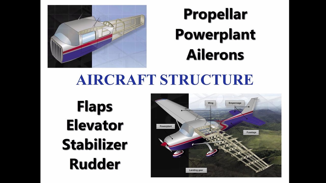
Private Pilot Tutorial 2: Aircraft Structure

A320 - Autoflight System (FCU - Flight Control Unit) PART 2
5.0 / 5 (0 votes)
