Lecture 22: Kernighan – Lin (KL) Algorithm

IIT Roorkee July 2018
8 Feb 202427:02

Summary

TLDRThis lecture introduces the Kernighan-Lin (KL) algorithm for VLSI Physical Design with Timing Analysis. It outlines the algorithm's steps, including initial partitioning, calculating cost functions, and iteratively swapping nodes to optimize partitioning. An example illustrates the process, demonstrating how to calculate 'D' values and 'delta G' for maximum gain, leading to a more efficient circuit partition. The lecture concludes with a discussion on the KL algorithm's time complexity, which is O(n^3), highlighting its significance in reducing cut costs and improving circuit design.

Takeaways

  • 📘 The lecture introduces the Kernighan-Lin (KL) algorithm, a method used in VLSI Physical Design for circuit partitioning with timing analysis.
  • 🔍 The KL algorithm is a multi-step process that begins with an initial partition and aims to minimize the cut cost by iteratively swapping nodes between partitions.
  • 🔢 The algorithm calculates a cost function 'd(v)' for each node 'v' to determine the balance of edges cut by the partition, which is crucial for evaluating potential node swaps.
  • 🔄 A key component of the KL algorithm is the 'gain' function, denoted as delta G(k), which is used to measure the potential reduction in cut cost from swapping nodes.
  • 🔝 The algorithm seeks to maximize delta G(k) by selecting the pair of nodes that provide the highest gain, thus reducing the overall cut cost.
  • ⏱️ The KL algorithm's efficiency is determined by two main factors: the evaluation of 'd' values and the computation of gain updates.
  • 🔁 The process iterates, with each iteration potentially fixing nodes that no longer need to be considered for swapping, thus reducing the computational load in subsequent iterations.
  • 📉 The algorithm continues until no further reduction in cut cost is possible, at which point all nodes are considered fixed, and the partitioning is complete.
  • 📊 The lecture provides a detailed example demonstrating the step-by-step application of the KL algorithm, including the calculation of 'd' values and the determination of the best node pairs to swap.
  • ⏳ The time complexity of the KL algorithm is O(n^3), primarily due to the gain evaluation process, which involves summing over a series that results in a cubic relationship with the number of nodes.

Q & A

  • What is the Kernighan-Lin (KL) algorithm?

    -The Kernighan-Lin (KL) algorithm is a heuristic algorithm used for partitioning a graph into two subgraphs with the goal of minimizing the number of edges that cross the partition, known as the cut cost.

  • What are the steps involved in the KL algorithm?

    -The KL algorithm involves several steps including initializing partitions, calculating cost functions, finding maximum gain for node swaps, fixing nodes, and iterating until no further improvements can be made.

  • How is the initial partition defined in the KL algorithm?

    -In the KL algorithm, the initial partition is defined with two sets, A and B, each containing an equal number of nodes, typically n nodes in each set.

  • What does the cost function 'd(v)' represent in the KL algorithm?

    -The cost function 'd(v)' represents the difference between the number of edges of a node 'v' that cross the partition and those that do not.

  • What is meant by 'delta G of k' in the KL algorithm?

    -'Delta G of k' is a cost function that measures the gain achieved by swapping two nodes between partitions A and B, defined as the sum of 'd(a)' and 'd(b)' minus twice 'c(a, b)', where 'c(a, b)' is the cost of edges between nodes a and b.

  • How does the KL algorithm decide which nodes to swap?

    -The KL algorithm decides which nodes to swap by finding the combination that yields the maximum 'delta G of k', indicating the highest potential gain in reducing the cut cost.

  • What is the purpose of fixing nodes in the KL algorithm?

    -Fixing nodes in the KL algorithm means that they will not be considered for swapping in future iterations, which helps to progressively converge towards an optimal partition.

  • What is the significance of the 'move sequence' in the KL algorithm?

    -The 'move sequence' in the KL algorithm is a series of node swaps that are accumulated to determine the overall gain after each iteration, guiding the decision to continue or terminate the algorithm.

  • How does the KL algorithm determine when to terminate?

    -The KL algorithm terminates when the overall gain 'Gm' becomes non-positive, indicating that no further reduction in cut cost can be achieved with additional swaps.

  • What is the time complexity of the KL algorithm?

    -The time complexity of the KL algorithm is O(n^3), which is determined by the number of times the gain function 'delta G' is evaluated, which happens in the order of n^2 times for each of the n iterations.

Outlines

00:00

💡 Introduction to VLSI Physical Design and KL Algorithm

The lecture begins with an introduction to the course on VLSI Physical Design with Timing Analysis, focusing on the Kernighan-Lin (KL) algorithm. The lecture's agenda includes discussing the KL algorithm's steps, using it for circuit partitioning, and analyzing its speed. The KL algorithm is broken down into multiple steps starting with an initial partition of nodes into two equal sets, labeled as 'a' and 'b'. The process involves calculating a cost function 'd' for each node and defining another cost function 'delta G' to determine the maximum gain for swapping nodes between partitions. The lecture emphasizes the iterative nature of the algorithm, where nodes are fixed as iterations progress until no nodes remain to be moved, leading to the final partition.

05:03

🔍 Detailed KL Algorithm Steps and Example Walkthrough

This section delves deeper into the KL algorithm's steps, using a practical example to illustrate the process. The example features a circuit with 10 nodes, initially partitioned into two groups with 5 nodes each. The lecture explains how to calculate the cut cost, which represents the number of edges crossing the partition boundary. The calculation of 'D of V' for each node and the subsequent determination of the maximum gain 'delta G' are discussed. The algorithm's iterative process is demonstrated, where nodes are swapped to optimize the partition, and the gain is accumulated. The example concludes with a discussion of how to determine the best iteration based on the maximum gain and how to decide when to stop the algorithm based on the sign of the accumulated gain.

10:04

📈 Algorithmic Efficiency: Gain Update and Pair Selection

The paragraph discusses the efficiency of the KL algorithm, focusing on two critical factors: gain update and pair selection. It explains how the number of times the cost function 'd' is evaluated decreases with each iteration, leading to an overall time complexity of O(n^2) for this part of the algorithm. The gain evaluation 'delta G' is also analyzed, showing that it is evaluated in a pattern that results in a time complexity of O(n^3). The paragraph concludes by emphasizing that the KL algorithm's speed is primarily determined by these two operations, with the higher complexity, O(n^3), being the dominant factor.

15:10

🔚 Conclusion and Algorithm Runtime Analysis

In the concluding part of the lecture, the instructor summarizes the steps of the KL algorithm and provides insights into its time complexity. The discussion highlights the importance of understanding the algorithm's efficiency for practical applications in VLSI physical design. The runtime analysis is reiterated, emphasizing that the KL algorithm operates at a complexity of O(n^3), which is crucial for assessing its performance in partitioning tasks. The lecture ends with a thank you note, acknowledging the audience's attention throughout the session.

Mindmap

Keywords

💡Kernighan-Lin Algorithm

The Kernighan-Lin Algorithm, often abbreviated as KL algorithm, is a heuristic algorithm used for graph partitioning. It is particularly useful in VLSI physical design for optimizing the layout of electronic components to minimize the number of connections crossing different regions. In the context of the video, the KL algorithm is the central topic, and the script describes its steps and application in circuit partitioning. The algorithm iteratively improves the partitioning to reduce the cut cost, which is the number of edges crossing the partition boundaries.

💡Partitioning

Partitioning in this context refers to the process of dividing a graph into two or more subsets or 'partitions' in such a way that optimizes a certain criterion, such as minimizing the number of edges that cross the boundaries between partitions. The script discusses how the KL algorithm is used to partition a circuit, starting with an initial partition and iteratively refining it to achieve a more efficient layout.

💡Cost Function

In the KL algorithm, the cost function is a measure used to evaluate the quality of a partition. Specifically, it calculates the 'cut cost,' which is the number of edges that cross the partition boundaries. The script mentions calculating the cost function 'd of v' for all nodes, which is a measure of how many edges of a node cross the partition. This function is crucial for determining which nodes to swap to improve the partition.

💡Gain (delta G)

Gain, or delta G, in the KL algorithm represents the improvement in partition quality that would result from swapping two nodes between partitions. It is calculated as the difference in cut costs before and after the swap. The script explains how to find the maximum gain to guide the swapping process, aiming to maximize the reduction in the cut cost with each iteration.

💡Iteration

An iteration in the context of the KL algorithm refers to a single pass through the algorithm's steps to refine the partition. The script describes multiple iterations, each starting with the calculation of 'd values' for nodes and ending with a decision to either continue with further iterations or terminate if no further improvement is possible.

💡Cut Cost

Cut cost is a key metric in graph partitioning that represents the number of edges that cross the partition boundaries. Reducing cut cost is the primary goal of the KL algorithm, as it directly impacts the efficiency of the circuit layout. The script provides an example where the initial cut cost is 11, and through the application of the KL algorithm, it is reduced to 1.

💡Nodes

In the context of the script, nodes refer to the individual elements of the graph that are being partitioned. The KL algorithm manipulates the placement of these nodes between partitions to optimize the layout. The script mentions that each partition starts with an equal number of nodes, and the algorithm iteratively fixes nodes' positions to minimize cut costs.

💡Edge

An edge in graph theory represents a connection between two nodes. In the KL algorithm, edges that cross partition boundaries contribute to the cut cost. The script discusses how the algorithm evaluates and minimizes the number of such edges to optimize the partitioning of a circuit.

💡Initial Partition

The initial partition is the starting point of the KL algorithm, where the nodes are divided into two partitions. The script explains that the algorithm begins with an even distribution of nodes, and through a series of iterations, it aims to improve upon this initial partition to reduce the cut cost.

💡Time Complexity

Time complexity in the context of the KL algorithm refers to the computational resources, particularly time, required to execute the algorithm. The script discusses the factors that influence the algorithm's speed, such as gain update and pair selection, and concludes that the KL algorithm has a time complexity of the order of n cube, where n is the number of nodes in the graph.

Highlights

Introduction to the Kernighan-Lin (KL) algorithm for VLSI Physical Design with Timing Analysis.

KL algorithm steps include initial partitioning, cost function calculation, and iterative improvement.

Explanation of Step 0 with initial partitioning into two sets A and B with equal numbers of nodes.

Step 1 involves calculating the cost function d(v) for all nodes and defining the gain delta G(k).

The process of finding the maximum delta G(k) to decide which nodes to swap between partitions.

Step 4 focuses on finding the move sequence 1 to m and calculating the accumulated gain G(m).

Criterion for continuing or stopping the algorithm based on the sign of G(m).

Example given with 10 nodes and initial partitioning, demonstrating the calculation of cut cost.

Detailed calculation of D(v) for each node and the subsequent selection of nodes for maximum gain.

Illustration of node swapping and its impact on cut cost and node fixation.

Explanation of the iterative process and how it continues until no nodes need to be moved.

The concept of gain update and pair selection as critical factors in the KL algorithm's speed.

Analysis of the time complexity of the KL algorithm, which is determined to be of the order of n cube.

Discussion on the practical application of the KL algorithm for partitioning circuits in VLSI design.

Conclusion summarizing the steps, example, and complexity of the KL algorithm.

Transcripts

play00:25

Welcome to the course on VLSI Physical Design with Timing Analysis.

play00:29

In this lecture, we will discuss about Kernighan-Lin or KL algorithm.

play00:35

The content of this lecture includes different steps of the KL algorithm, then we will discuss

play00:42

partitioning of a circuit using KL algorithm.

play00:45

We will take an example and discuss how the KL algorithm is useful for partitioning.

play00:51

Then we will discuss about the what is the speed of speed of running the KL algorithm.

play00:58

So, this KL algorithm has multiple steps, we will discuss one at a time.

play01:03

So, step 0 is basically we have a initial partition.

play01:09

So we have a initial partition and see this a and b are the two partitions and your number

play01:16

of node is or the number of vertices is basically 2N.

play01:21

So a has n nodes, a or b has n nodes.

play01:31

So each partition has same number of nodes.

play01:35

So then we will go to the step 1.

play01:37

In the step 1, we have k equals to 1.

play01:40

So here we have to calculate the cost function d of v. For all nodes v belongs to v. So here

play01:48

we need to let us say we have 2N nodes, we have to calculate the v of v 2N times for

play01:57

one time for each node.

play02:00

So now after we find out basically v of each node, then we will define another cost function

play02:09

that gain delta G of k.

play02:13

So this is delta G of k which is defined as d of a plus d of b minus 2 c (a, b).

play02:24

c (a, b) is a comes when there is a edge between a and b.

play02:31

So we need to find out where my delta G of k is maximum.

play02:36

So then only we can swap a and b and we will not change that a and b in the next iteration.

play02:47

So in this process every iteration we are fixing 2 nodes because after the swap we are

play02:54

fixing those nodes.

play02:56

So the time will come when there is none of the nodes need to be moved.

play03:01

There is no nodes means all the nodes will be fixed.

play03:05

If all the nodes are fixed then we have to go to the step 4.

play03:09

Otherwise we will compute the d values for each node connected to a and b which are not

play03:16

fixed then we will increase the value of k plus 1 then we will go to step 2.

play03:22

Step 2 will do what?

play03:24

It will find the delta G of k this one.

play03:30

For all possible combination of the nodes which are not fixed then we will find out

play03:37

which is giving me the maximum gain maximum value of delta G then that will be taken for

play03:44

moving from one partition to other and those nodes will be fixed.

play03:49

So this process will continue till all the nodes are fixed then we will go to the step

play03:57

4.

play03:58

In this step 4 we will find a move sequence 1 to m.

play04:03

So m is something between 1 to k and each m it is basically accumulation of previous

play04:15

gain we are doing the accumulation of the previous gains.

play04:20

So your delta G of k will be G of m is summation k equal to 0 to m delta G of k.

play04:28

If your Gm is greater than 0 then you go to step 5.

play04:39

Greater than 0 means if your Gm is positive.

play04:42

If your Gm is positive then you have to continue the process will continue.

play04:51

If Gm is negative then stop.

play05:03

So these are the two case 1 and case 2.

play05:10

So then execute m swaps and reset the remaining nodes and go to step 1.

play05:15

So this is for the step 5.

play05:18

Now we will take an example and see how these things are happening.

play05:22

So this is the first path.

play05:24

So this is basically having basically your number of nodes V equals to 10 here.

play05:36

So your V is 10 here and you have a partition A this side is let us say partition A this

play05:43

side is partition B. So each one of them are having 5 nodes and all the nodes or vertices

play05:52

are not fixed all the nodes 1 to 10 are not fixed.

play05:58

Then how many cut cost is there?

play06:00

How many this is the cut line.

play06:03

Cut cost is basically the number of edges passing through the cut lines.

play06:11

So here if you have seen 1, 2, 3, 4, 5, 6, 7, 8, 9, 10, 11.

play06:25

So number of cuts cost is 11.

play06:29

So now we will go to calculation of D of V. So whenever I am calculating D of V in the

play06:35

first k equal to 1.

play06:39

So how many times I need to calculate D?

play06:42

Number of times the D is evaluated at this k equals to 1 is 10 which is proportional

play06:58

to 2N which is proportional to 2N.

play07:04

Now let us say how the D's are evaluated.

play07:06

First we will calculate the how the D's are evaluated.

play07:09

Let us take the node 1.

play07:13

Node 1 if you can see here I have 1, 2 and 3 edges.

play07:21

So the 1 and 2 are passing through the cut line and the 3 which is the which I wrote

play07:27

in the blue color is not passing through the cut line.

play07:30

So my D of 1 is basically 2 minus 1 is 1.

play07:41

Similarly I can calculate for any other node D of 9.

play07:45

Let us say this 9.

play07:48

So D of 9 is basically here 1, 2, 3 are the edge cut by the cut line which is 3.

play08:01

Then this edge is not cut by the cut line.

play08:03

So this will be 1, it will be 2.

play08:06

D of 9 is 2.

play08:08

So we have to calculate for all the D's.

play08:11

So now I need to choose which is giving me maximum gain delta G. So if you can see here

play08:17

ideally you have to do it for all the combinations but here looking at this evaluation I can

play08:25

see D of 2 and D of 9 has cost of D of B is highest.

play08:36

So let us take those nodes for gain calculation or moving from one partition to the other.

play08:44

So if I take these two nodes D of 2 is 2 and D of 9 is 2 here my gain because there is

play08:54

a 2 and 9 there is no edge between them C of A, B is 0.

play08:59

C of A, B at this point is 0.

play09:03

So now delta G of 1 is 2 plus 2 minus 0 which is 4.

play09:12

Now this 2 and 9 should be swapped.

play09:20

My gain is basically G of 1 is delta G 1 because it is a first iteration it is 4.

play09:28

After we do this then which node will be fixed?

play09:32

The 2 and 9 will be fixed.

play09:34

In this case 2 and 9 are swapped so the 2 and 9 are fixed and rest of the nodes are

play09:44

not fixed.

play09:48

So we have 8 nodes not fixed, 2 nodes are fixed in iteration 1.

play09:56

Now we will calculate D of B of each node.

play10:04

So if you can see here if I look into this D values the number of times the D is evaluated

play10:19

is basically 2N minus 2K.

play10:30

So 2N in this case is 10 minus 2 which is 8.

play10:36

So you have number of times your D is evaluated is 8.

play10:42

So 1, 2, 3, 4, 5, 6, 7, 8.

play10:48

So now we can see which of the nodes will be swapped.

play10:55

If you can see here D of 1 is giving me a gain of 3 and D of 10 is giving me a gain

play11:06

of 3.

play11:08

So these two nodes are showing is basically giving highest gain.

play11:13

So I need to swap them.

play11:16

So ideally you have to do it for all nodes if you are doing algorithm but here we are

play11:23

visually finding the nodes.

play11:26

So this node 1 and 10 need to be swapped.

play11:30

So now in this slide if you can see so the C of 1, 10 because node 1 and node 10 there

play11:40

is no edge between them so this is 0.

play11:43

So the gain this will be 0 because of this, this 3 is coming because of this 3 and this

play11:50

3 is coming because of this 3.

play11:51

So my delta G2 is basically 6 here.

play11:55

Now I need to accumulate all the previous gain with this present gain.

play12:01

So my previous gain is basically G1 plus delta G2.

play12:06

So my overall gain is basically 10.

play12:10

So now my number of cut cost will be reduced by 10 after doing this move of these two nodes.

play12:20

Now if I can see I have 4 nodes are fixed, 1, 2, 9, 10 are fixed and the rest of the

play12:28

nodes are not fixed.

play12:32

So here the K is basically 2 here.

play12:35

So now we have 4 nodes fixed, 6 nodes are not fixed.

play12:40

So now if I can see number of times D is evaluated in this iteration is basically 2N minus 2

play12:56

into K.

play12:58

So basically if you can see 10 minus 2 into 2 here it is 6.

play13:07

So you have 4 nodes are fixed for them you do not need to calculate the D but rest 6

play13:15

nodes you need to calculate the D. So 3, 4, 5, 1, 2, 3, 4, 5, 6 I need to calculate the

play13:25

D. See if I can look into this which node is giving me the best swap is basically all

play13:33

are negative.

play13:34

So the maximum negative number will give me the best swap.

play13:39

So the 3 and 8 nodes are chosen actually minus 1, D of 3 is minus 1, D of 8 is minus 1.

play13:49

So if I do this my gain is now basically minus 4 means I am not getting any improvement in

play13:57

the cut cost if I go by this.

play13:59

However, I have to check if I can get a better solution in the future.

play14:03

So your G3 is basically G2 plus delta G3 which is giving me 6.

play14:12

So now this is the new partition after this iteration.

play14:17

If I can see I have basically fixed node 1, 2, 3, 8, 9, 10 these are the fixed nodes and

play14:27

these 4 are not fixed nodes we need to calculate the D's for them.

play14:32

So number of times D is evaluated is basically 2N minus 2 into K.

play14:49

So 2N is basically 10 minus 2 into 3.

play14:53

So this will give me basically 4.

play14:57

So here you have 1, 2, 3, 4.

play15:01

So D is evaluated for the on fixed nodes 4, 5, 6, 7 in this case.

play15:10

Now that once the D is evaluated then I have to choose pair of nodes to get a maximum gain.

play15:15

So in this case if I can see 4 and 7 will give me the maximum gain.

play15:20

So the 4 and 7 is chosen.

play15:24

Now the gain becomes G4, the delta G4 is basically minus 4.

play15:33

My cumulative gain is basically G4 is basically 2.

play15:40

So this is after doing this pass my all of the nodes which are fixed is basically 8 nodes

play15:49

are fixed and 2 nodes are not fixed.

play15:55

So then I need to calculate the D for the 2 nodes.

play15:59

Number of times the D is evaluated is basically 2N minus 2 into K.

play16:14

So 2N is basically 10 minus 2 into 4.

play16:20

So this number of times the D is evaluated is 2, this is 1, this is 2.

play16:26

So for these 2 on fixed nodes we need to help calculate the D. So there are 2 options, only

play16:33

1 pair of nodes are there.

play16:35

We do not have any choice.

play16:37

So we have to choose these 2, 5 and 6 for the swap.

play16:42

So after you do the swap my gain becomes 0 here.

play16:47

There is no improvement in the cut cost whatever the 11 cut cost was there.

play16:52

Now the same cut will come at the final cut.

play16:55

So there is no improvement.

play16:58

Now we have this final step where K equals to 5.

play17:03

I have total cut cost is becoming 11 and all the nodes are fixed and I do not have any

play17:10

node to do D's evaluation.

play17:14

So I have basically iteration K equal to 1, K equal to 2, K equal to 3, K equal to 4 and

play17:21

K equal to 5.

play17:22

My x axis is basically K and y axis is basically my gm.

play17:29

So if I plot this one which iteration is giving me maximum gain that I should choose.

play17:39

So if you can see here my K equals to 2 is giving me my maximum gain.

play17:45

So this is corresponding to this node, this point in the graph.

play17:52

So that is the best choice.

play17:56

So if you can see here my gm is greater than 0 and the first m equal to 2 because first

play18:02

2 swap I am getting the best result.

play18:06

So in the K equals to 1, the 2 and 9 nodes are interchanged or swapped and K equals to

play18:17

2, my 1 and 10 nodes are swapped.

play18:26

So this is my final partition after the pass one.

play18:32

So if I can see here my gain is positive.

play18:35

I need to iterate it till my gain is negative.

play18:40

So since my gain is positive more paths are needed until my gain is negative.

play18:46

gm should be less than equals to 0.

play18:50

So I have to go to the second pass.

play18:53

So the output of the first pass is the initial partition for the second pass.

play19:00

So here the cut cost is 1 and I have all the 10 nodes are unfixed.

play19:09

So the same procedure whatever was followed in the pass one the same procedure will be

play19:15

repeated here.

play19:18

So I have to calculate all the d's and from them which is giving me the best result that

play19:24

will be best gain that will be taken and swapped.

play19:28

So that method will be followed.

play19:33

So I am not discussing all the steps but this is the results for K equals to 2 and the gain

play19:47

is K equal to 2 is basically your g is basically minus 8.

play20:05

So here what is the basically your K values are your x axis is basically K and gm is basically

play20:15

your y axis for different values of K.

play20:19

So if you can see here your gain is becoming negative and finally it is settled to 0.

play20:27

So since your gain final gain and all the gains are negative so I can stop my algorithm

play20:33

here I do not need any further pass.

play20:36

So since I am gain overall gain is 0 so this is my initial partition my gm is there is

play20:46

no gm is 0 finally and so there is no further passes are needed we can terminate the algorithm

play20:54

here and this is my final partition.

play20:57

And in this case my cut cost was 11 now in this final partition the cut cost is become

play21:09

1.

play21:10

So, this is the final partition is the best partition because I have reduced the cut cost

play21:16

by 10.

play21:17

Now we will discuss about the runtime of the K-L algorithm.

play21:22

So this runtime will tell my speed of a pair algorithm how fast my algorithm is working.

play21:28

So the K-L algorithm is basically determined the speed of the algorithm is determined by

play21:34

two factors one is my gain update and the pair selection.

play21:39

So we will discuss how the algorithm speed depends during the gain updates and the pair

play21:46

selection.

play21:47

So here we have basically that so if I have whatever I discussed in the first iteration

play21:58

K equal to 1 I have to evaluate d basically 2n times K equal to 2, my d is evaluated basically

play22:12

2n minus 2 basically this the first one is 0 and this is K equals to 1.

play22:23

So I have basically 2 K so it will be evaluated 2 times less than the 2n.

play22:32

So similarly, if I go in this method finally the d will be evaluated 0 times.

play22:39

So here what is happening is that my 2n, 2n minus 2i like that it is going.

play22:46

So now basically what is happening is that my d number of times the d is evaluated is

play22:53

reduced by 2 in each iteration.

play22:57

So if I make a sum of that because how many times the K should run?

play23:05

How many times the K should run?

play23:09

The K should run for number of nodes by 2 which is n.

play23:18

So that is why your this is this n comes into picture.

play23:22

So you have a summation I equal to 1 to n 2n minus 2i.

play23:31

So i is basically index for K.

play23:35

So now this is basically order of n square.

play23:42

Now we have basically your gain evaluation delta G. So the delta G is evaluated how many

play23:52

times?

play23:54

When the K equals to 1 the delta G is evaluated how many times?

play23:58

The delta G is evaluated 25 times.

play24:03

So it is basically n square.

play24:11

Your number of nodes is 2n and n is basically half of the nodes actually.

play24:18

So when K equal to 2 your delta G is evaluated how many times?

play24:23

It will be basically 4 this side 4.

play24:28

So 16 times, n minus 1 square like that.

play24:34

So how long it should run?

play24:36

It should run till basically 5.

play24:39

So your delta G will be running 1.

play24:47

So it will be 1.

play24:50

So basically if I can have total number of times the delta G is evaluated basically n

play24:56

square plus n minus 1 square n minus 2 square dot dot dot 1.

play25:05

So this we can represent it in a series as this one we can represent this one we can

play25:13

represent as a series as summation i equal to 1 to n, n minus i plus 1 whole square.

play25:25

So this is basically because already one square is there there is another loop is there so

play25:29

it is order of n cube.

play25:33

So we have two operation we are doing one is de-evaluation is doing one is your gain

play25:39

evaluation your delta G evaluation de-evaluation is happening or order of n squares and this

play25:49

gain evaluation is happening order of n cube.

play25:52

So it is out of both which is the highest that is order of n cube.

play25:58

So the speed of this algorithm is basically order of n cube.

play26:03

In this lecture we discuss about the steps of the KL algorithm we discuss also about

play26:10

one example how we can find out the D and delta G to find a final partition using the

play26:18

KL algorithm.

play26:19

Then we discuss about the complexity of the KL algorithm how it is useful we should know

play26:25

the time complexity of the algorithm.

play26:27

So we discuss that in detail.

play26:29

Thank you for your attention.

Rate This

5.0 / 5 (0 votes)

Related Tags
VLSI DesignKL AlgorithmCircuit PartitioningTiming AnalysisAlgorithm ComplexityElectronic EngineeringEDA ToolsOptimization TechniquesDesign AutomationComputer Science