Plant Leaf Disease Detection Using CNN | Python

Summary

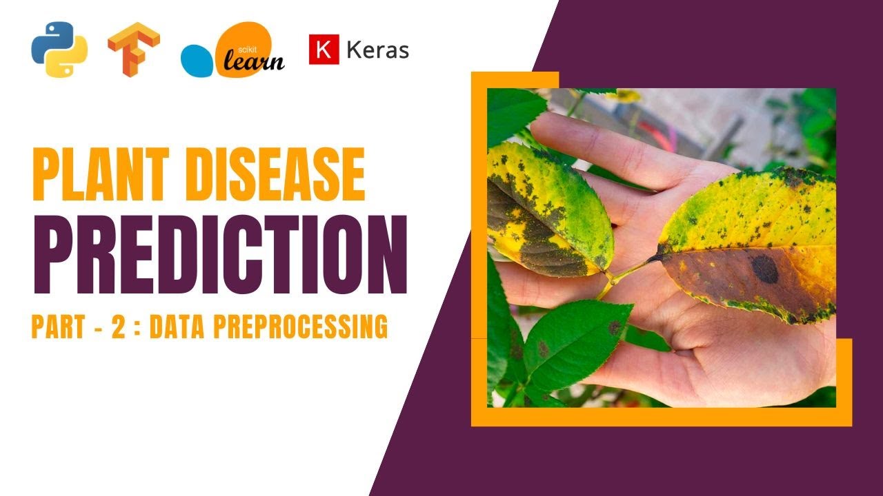
In this YouTube tutorial, the host demonstrates how to build a deep learning model for plant disease classification using Python and TensorFlow. They showcase a demo application that predicts leaf diseases from images, utilizing a dataset from Kaggle. The video guides viewers through the process of creating a CNN model, training it with image data augmentation, and compiling it for accuracy. The host then explains how to deploy the model into a web application using Flask, allowing users to upload images for disease prediction. The tutorial is practical, providing step-by-step coding instructions and emphasizing the importance of data balance and model evaluation.

Takeaways

• 🌟 The video is a tutorial on building a deep learning application for plant disease classification using Python and the Flux web framework.
• 🔍 The demo application allows users to upload images of plant leaves and receive predictions on diseases like rust and powdery mildew.
• 📁 The tutorial uses a dataset from Kagle, which includes training, testing, and validation sets with images categorized as healthy, rust, or powdery.
• 💾 The data is already split into these sets, so there's no need for additional data partitioning by the user.
• 🔄 The script discusses the importance of data augmentation to increase the dataset size and improve model training, using techniques like image rescaling and flipping.
• 🤖 The model used is a Convolutional Neural Network (CNN) due to the image-based nature of the data, with layers including convolution, max pooling, and fully connected layers.
• 📈 The tutorial covers the process of compiling the model with categorical cross-entropy as the loss function, using the Adam optimizer, and training the model with a specified batch size and number of epochs.
• 📊 The video includes a demonstration of the accuracy and loss curves to evaluate the model's performance and ensure it is neither overfitting nor underfitting.
• 🖼️ The process of pre-processing new images for prediction involves resizing, normalization, and expanding dimensions to match the model's input requirements.
• 🛠️ The video concludes with instructions on building a web application using the trained model, including setting up routes and handling image uploads and predictions in a Flask application.
• 🔗 The source code and additional resources for the web application are available in the video description or on GitHub for further exploration and use.

Q & A

What is the main topic of the video?

The main topic of the video is building a deep learning application for plant disease classification using Python and TensorFlow.

What is the purpose of the demo application shown in the video?

The purpose of the demo application is to classify plant leaf diseases by predicting whether a leaf is healthy, affected by rust, or has powdery mildew based on images.

What dataset is used in the video for building the deep learning model?

The dataset used is from Kaggle called 'Plant Disease Recognition' which contains images divided into training, testing, and validation sets for three classes: healthy, powdery, and rust.

What are the three classes of plant diseases considered in the dataset?

The three classes of plant diseases considered are healthy leaves, leaves with powdery mildew, and leaves with rust.

Why is data augmentation used in this context?

Data augmentation is used to increase the amount of training data by creating new images from existing ones through techniques like rescaling, shearing, zooming in/out, and horizontal flipping, which helps in improving the model's generalization.

What type of model is being built in the tutorial?

A Convolutional Neural Network (CNN) model is being built in the tutorial, which is suitable for image data.

How does the video demonstrate the model's performance?

The video demonstrates the model's performance by showing the accuracy on the training and validation sets, as well as by plotting accuracy and loss curves.

What activation function is used in the final layer of the CNN model?

The Softmax activation function is used in the final layer of the CNN model because it is a multiclass classification problem.

How can the trained model be utilized in a web application?

The trained model can be saved as a file (e.g., model.h5) and then integrated into a web application using a framework like Flask, where users can upload images to get predictions.

What is the significance of the 'pre-process_image' function in the context of the video?

The 'pre-process_image' function is significant as it prepares the images for the model by resizing them to the required input size of the CNN, converting them into a NumPy array, and normalizing the pixel values.

How does the video ensure the model is not overfitting or underfitting?

The video ensures the model is neither overfitting nor underfitting by comparing the accuracy on the training set with the validation set and by showing that there is no significant gap between the two, indicating a well-generalized model.

What is the role of the 'secure_file' in the web application code?

The 'secure_file' role in the web application code is to prevent unauthorized file access, ensuring that only approved files can be used within the application.

Outlines

00:00

🌿 Introduction to Plant Disease Classification with Deep Learning

The video begins with an introduction to a project on plant disease classification using deep learning. The presenter demonstrates a Python and Flask application that can identify diseases in plant leaves by analyzing images. The application uses a dataset from Kaggle, which contains images of healthy leaves and those affected by powdery mildew and rust. The presenter guides the audience through the process of choosing images, predicting diseases, and emphasizes the importance of building the model from scratch using Python, deep learning, and Flask.

05:00

🔍 Exploring Data and Setting Up the Deep Learning Model

The second paragraph delves into the details of preparing the dataset for the deep learning model. The presenter explains the process of loading data, checking for balance or imbalance, and creating functions to facilitate data retrieval and counting. The audience is introduced to the concept of data augmentation to increase the dataset's size using an image data generator. The paragraph also covers the initial steps of building a Convolutional Neural Network (CNN) model, including the selection of layers and activation functions, and the importance of compiling the model with the appropriate loss function and optimizer.

10:00

🚀 Training the Deep Learning Model and Evaluating Performance

In this segment, the presenter discusses the training process of the deep learning model, including setting the batch size and epochs. The video script mentions the use of a validation set to monitor the model's performance and avoid overfitting. The presenter also explains how to visualize the accuracy and loss curves to assess the model's learning progress. The paragraph concludes with instructions on how to save the trained model for future use and how to test the model with new data by preprocessing the images to match the model's input requirements.

15:02

🌐 Building a Web Application for Disease Prediction with Flask

The fourth paragraph outlines the process of creating a web application using Flask to deploy the trained deep learning model. The presenter describes the structure of the web application, including the creation of folders for static files, templates, and the main application code. The video script provides an overview of the code involved in setting up the routes, handling file uploads, preprocessing images, and using the model to make predictions. The presenter ensures that the application is secure and user-friendly, allowing users to upload images and receive predictions on the fly.

20:03

📚 Conclusion and Testing the Web Application

The final paragraph wraps up the tutorial with a conclusion and a live demonstration of the web application in action. The presenter shows how to run the application on a local server and test it with various images to see the prediction results. The video script emphasizes the successful implementation of the project and encourages viewers to subscribe to the channel for more content. The presenter also hints at future tutorials and thanks the audience for watching.

Keywords

💡Deep Learning

Deep Learning is a subset of machine learning that uses artificial neural networks with multiple layers to model and understand complex patterns in data. In the context of the video, deep learning is utilized to classify plant diseases from images, demonstrating its application in image recognition tasks. The script discusses building a deep learning model using Python, which is a common programming language for such applications.

💡Flux

Flux, in the context of this video, likely refers to a web framework for building web applications in Python. The script mentions using Flux to create a web application that allows users to upload images and receive predictions from the deep learning model about plant diseases. This showcases how deep learning models can be integrated into web applications for practical use.

💡Plant Disease Classification

Plant Disease Classification is the process of identifying the type of disease affecting a plant based on visual or other data. The video's main theme revolves around this concept, where a deep learning model is trained to classify images of plant leaves into categories such as 'healthy', 'powdery mildew', and 'rust'. The script provides a walkthrough of how to predict and classify these diseases using a deep learning model.

💡Data Set

A Data Set in this video refers to a collection of data used for training and validating the deep learning model. The script mentions a specific data set from Kaggle called 'Plant Disease Recognition', which contains images categorized into 'healthy', 'powdery', and 'rust' classes. This data set is fundamental to the model's training and evaluation process.

💡Model Training

Model Training is the process of teaching a machine learning model to make predictions or decisions based on a dataset. In the script, the process involves using a deep learning model to learn from images of plant diseases. The training process is crucial as it determines the model's ability to accurately classify unseen images.

💡Convolutional Neural Network (CNN)

A Convolutional Neural Network, or CNN, is a type of deep learning model that is particularly good at processing data with a grid-like topology, such as images. The script describes building a CNN model for the task of image classification in plant disease detection. CNNs are chosen due to their effectiveness in capturing spatial hierarchies in image data.

💡Data Augmentation

Data Augmentation is a technique used to increase the amount of training data by creating modified versions of the original data. In the video script, this technique is used to artificially expand the image dataset by applying transformations like rotation, zoom, and horizontal flip to the images. This helps in improving the model's generalization and reducing overfitting.

💡Epoch

An Epoch in machine learning refers to one complete pass through the entire training dataset. The script discusses training the model for a certain number of epochs, which is important as it affects how well the model learns from the data. More epochs can lead to better learning but also increase the risk of overfitting.

💡Accuracy

Accuracy in the context of this video refers to the measure of how correctly the model predicts the class of the images. The script mentions achieving a certain percentage of accuracy on the training and validation sets, indicating the performance of the model. High accuracy is a desirable outcome in model training.

💡Web Application

A Web Application, as discussed in the script, is a program that allows users to interact with the deep learning model through a web interface. The video demonstrates how to build a web application using the trained model to predict plant diseases from user-uploaded images, showcasing the practical application of deep learning in a user-friendly format.

💡Image Preprocessing

Image Preprocessing is a series of operations performed on an image to prepare it for further analysis or modeling. In the script, preprocessing includes resizing images to match the input size expected by the CNN model and normalizing pixel values. This step is essential for ensuring that the input data is in the correct format for the model to process effectively.

Highlights

Introduction to a YouTube tutorial on building a disease classification application for plants using deep learning with Python and TensorFlow.

Demonstration of the application's ability to classify plant diseases from images with high accuracy.

Explanation of the dataset source from Kagle, containing images of plant diseases for training, testing, and validation.

Description of the data set's structure with three classes: healthy, powdery, and rust.

Tutorial on creating a function to load and count the data for balanced or imbalanced assessment.

Use of the ImageDataGenerator for data augmentation to increase the dataset size.

Building a Convolutional Neural Network (CNN) model with TensorFlow's Sequential model.

Inclusion of layers such as Conv2D, MaxPooling, Flatten, and Dense with the Softmax activation function for multi-class classification.

Compilation of the model with categorical cross-entropy loss, accuracy metric, and the Adam optimizer.

Training the model with a batch size of 32 and for 5 epochs, including validation data.

Analysis of the accuracy curve to ensure the model is neither overfitting nor underfitting.

Instructions on saving the trained model for future use.

Process of testing the model with new images and pre-processing them for prediction.

Building a web application using Flask to deploy the model for practical use.

Explanation of the Flask application structure including templates, static files, and routing.

Integration of the pre-trained model into the Flask app for making predictions from uploaded images.

Demonstration of the web application in action, classifying new images of plant diseases accurately.

Encouragement for viewers to subscribe to the channel and look forward to future content.

Transcripts

hello everyone and welcome back to my

YouTube channel and in this video we are

going to be discussing about the planned

disease classifications using deep

learning and this is De application buil

by using Python and flux so let's see

the demo application first so first I'm

going to click at to choose the file and

choose on the picture from my directory

testing folder I'm going to select the

pictures and click at to open and click

at to

predict and this is the healthy Leaf

healthy leaf plant if I select another

photo let's say I'm going to select the

photo from the rust and let's select

this one click on open and if I predict

and you can see here this is nothing but

the rust so if I select another

photo from my another directory is

called powder so this is one kind of dis

is plant that's called the powdery and

it's also PR it

correctly now in this Tut we're going to

build this full application from the es

course using deep learning Python and

flux so without wasting any time let's

start the tutorial now so in order to

build in the full application we're

going be using a data set from kagle

that's called the plant disease

recognization data set which are

containing three files called the train

test and the abilitations and each

folder containing three files or you can

say the number of classes first one is

called healthy second one is called the

powdery and third one is a rust Now

using this data set we going to building

our deep learning model and after that

we're going to building our web

applications using flux so now what we

going to do you just need to create your

own account on that and after that you

can click on the download and download

the data set on your directory so well

so this is the code for that and I draw

the code in my J notebook you can also

do it in BS code or the py term or

Google Cola itself if you don't have any

much more amount of GPU so I going to

explain all the code line by line so

that you don't need to worry about that

what actually happening inside this code

and you also building our deep learning

model don't worry on that so now I'm

going to start the tutorial now and

explaining all the code line by line so

first what you need to do you need to

load the data from our data set folder

right and also need to check that if our

data is Balan or imbalanced right so

first what we can do we can simply

create here functions which can actually

help us to get the data from here and

also do the counting right so for that

we to import the O then you need to

create here a function that's called da

total files and you create here a Lambda

function and which one actually creating

the list of the each folder each folder

and give here the length right so for

that you need to give here path let's

called the training file healthy the

powder and the rust so this is nothing

but my classes I mean how many classes

are available inside our data set folder

so you have the three classes healthy

powdery and rust so it simply actually

give you the path of that data set we to

go in the train then train and healthy

right so this is the path for that and

again the path for the test file and

also the abilitation file simple then

what I can do you can simply print it

out so you can run the code from here

and also you can use the shortcut

technique that's called the shift and

the the enter in the keyboard shift and

the enter and to run the code

automatically so you can see number of

the healthy images are training set is

458 right and you can see the testing

set and also the bation set so now let's

have a look the data first so let's say

look one healthy images so this is the

healthy leaf images quite good right so

let's see also the r one I mean the

affected one so this is the r images

with having some spot with having red

and the black so what we going to do

we're going to Simply classify them

which one is a good leap or which one is

a bad leap right or which one is a

powdery leap right so see we have the

limited amount of data and also one more

important thing in every video when

you're building the machine learning or

de learning model we need to divide the

data into the train test and split but

in this data set you need to do you

don't need to do that because the kaggle

authority actually do this code again I

mean the data set uh the person or the m

number actually building the data set he

actually do this already right you can

see the training set the testing set and

the validation set that's me he should

divide the data set in the train test

and the validation already you don't

need to do it you you don't need to do

it so that's one plus point for you so

now what we can do we can simply do the

data argumentation now the question is

what is data argumentation and why you

need to do that see we have the limited

number of data just less than 500 less

than 500 so how can we do the data

documentation in the Deep learning how

can you do that yes we can do it is with

the same images using some technique

using some technique that's called the

image data generator so which one

rescale the images which one give you

the sharing and we can also zoom in or

zoom out and do the horizontal flip and

create some new images create some new

images in your HEAP memory in your

memory in your memory right it don't

actually store in your your folder it

will actually store it in the memory so

let's say I have the 400 images so it

will generate let's say 300 images so

total 700 images that's mean if you give

here the 500 images it will generate

more 300 or 400 and create a model for

that create a model for that that's

called the image data generator or you

can say the data argumentation so what

you can do you can simply using his

image data generator and create a object

for that and it will take some parameter

to rescale this and after that you're

going to give here our image data

generator right so we actually creating

the object for that now what we can do

we can simply run the shell and after

that you're going to apply it in our

full data set we're going to apply it in

our full data set so we have the three

folder train test and the validation so

we're going to using the training set

and the validation set then using this

test set you're going to checking for

the accuracy you're going to checking

for the accuracy so for what you going

do we can simply flow from the directory

see one more thing flow from the

directory how you actually use it how

you get one data set which one is

already divided into train test and

split if you're trying to flow from the

directory and also do the data

argumentations using this one that's

called a flu from directory that's mean

when you are passing your data inside

your image data generator you need to

use this flu from directory so taking

the all images from your directory and

create and create one extra create one

extra uh you can see extra directory

forther right in your memory so you can

see found 100 322 images belong three

classes it have the three classes right

it will automatically throw the data

from your directory you don't need to

use the West you don't need to use the

globe don't worry and you can see we got

here the 100

1,322 images which one the actual images

which one the actual images it have also

the image data generator images but it's

not showing up here it's not showing up

it is stor in our memory it is stor in

our memory now what we can do we can

simply building our deep learning model

or you can CNN model now which kind of

model are you going using here obviously

CNN because this is a image data if it

is a numerical data you can use the Ann

or the RNN or the lstm right based on

your data set if it is if it is time

series types of data you can obviously

use the lstm or the RNN right so now

what you can do you can simply building

our deep learning model or can CNN model

so we going building here sequential

model so there are two types of model

are available sequential and another one

is called the functional so sequential

mean you're going passing the data from

one layer to another layer and do the

conation operation and do the conation

operation so for import the caros do

model import the sequential then uted

the cony the max pulling layer so there

are so many Max pulling Factor actually

available Max pulling 2D the average

pulling

right available right so you can see the

flatten so flatten what actually do when

you give your data it's a multi

dimensional data multi-dimension mean so

many dimensions so when you pass it

inside your CNN model you need to give

it in one kind of vector just a single

Vector so that's using the flatten and

Dance is for the final layer the input

or the output layer right so first you

going to create here the sequential we

actually give here my kernel uh 32 right

3 2 and 3 cross three filter and input

shape is 225 225 3 so 225 is mean height

and the weight and three is number of

channel number of Channel and we have

the activation function that's called

the reu so reu is actually the formula

of re is a Max of Max of Z comma J right

Max of Z comma J that mean you're taking

the maximum value it will taking the

maximum value then what you can do we

can simply give you the pulling the max

pulling having the pool size of the two

it will taking the maximum value for the

each full ch right then we going to give

here the 64 again 64 activation Rel

activation function and add here on

maxing layer then finally you going to

use here the flatten layer I mean

creating here one single vector and give

you the dance layer of the 64 and dance

layer of the three so three is nothing

but my number of classes I mean how many

classes are available in your data set

we have three classes we have three

classes so that's put here three and

activation function is soft Max so

because this is the multiclass

classifications so that's why you give

here the soft Max otherwise you can give

here

we can give you the sigma then need to

to also compile the model so before you

fitting or you can training the model

you need to also compile it see one more

important thing we give your law as a

categorical cross entropy so when you

have multiclass classification types of

project it give here the categorical

cross enty if it's a binary

classification it should be the binary

cross enty and Matrix is same accuracy

and Optimizer is Adam you can also use

gradient Des set S2 gr also you can also

do it right so now what you can do you

can simply compile it and after that

after compiling you need to you need to

OKAY model is defined I need to we need

to also run this shell so that's why and

we need to compile it now and after

compiling we need to we need to train

the model we need to train the model and

you can see the bass size is 16 right

you can also give a 32 it's up to you

right it's based on your system

requirement right you also let's give

here the 32 right now and epox is right

now five AO is right now five and

validation data you can give here the

validation from it's coming from the

validation generator and the validation

b side let's say 16 so if I go here it

just have that 20 Imes so it's better we

can give you the B size of 16 right

because we have the low amount of data

so that's why you can also give it 32 or

the 64 it's up to you so now what I'm

going to do I'm going to Simply run the

code and start the epox so what actually

epox epox me should go from the forward

propagation and again go to the back

propagation and actually calculate the

weight and based on the weight it will

actually minimize this weight minimize

the cost function or you can minimize

the weight so that's called the eox I

mean One For What and one backward and

update the weight and update the weight

so this is nothing but called the epox

so after that what you going do uh we

can also generate here one figure for

that this is called the accuracy curve

so I'll back again when the training

part is completed right so well so our

model training is completed and you can

see here I got here the 90% % accuracy

and the validation accuracy is 88% so if

I trying to click here to run this shell

to floting the accuracy curve and the

loss curve and you can see here uh our

model is working really fine it's not

over fitting or underfitting data uh

because it's it don't have any Gap right

now right that's when our model is

working really very fine so you can also

increase your epox in order to also

increase your accuracy we got here the

90% accuracy you can also increase it by

increasing the epoch number right right

so now what I can do I can simply going

to save the file in a model file model.

as5 so that we can use it in the later

on or you can also use it in your own

devices also so now what we can do we

can simply test it out we can simply

test it our new data so I'm going taking

one image from the rust in our directory

then after we testing out right so

forther what you need to do you need to

also load the images same as it is we do

in our data set and after that you need

to convert this image into the number

ARR so so we going to create here a

function which will actually give here

the pre-process image so first you

loading the images with having the

target size of 225 cross 225 because if

I go up in our uh CNN model we give here

the input shape is 225 2253 so that's

why you need to also resize the images

in this uh kind of sizes 225 plus 225

then we are going to pass it inside our

image to AR image to actually do you

convert this image into one n AR so that

we we can actually normalize it we can

normalize it and you can see here it

should divide the data into 255 so why

255 actually if you see one images gray

scale gray scale or the RGB images let's

say RGB images it have the value

starting from 02 255 so if I'm trying to

normalize the data between zero and one

we divide the data into big number the

maximum number you can see the maximum

number so the maximum number is 2555 so

that's why divide the data using the 255

then we dra the expand Dimensions to the

expand the dimension of the data so that

we can get our actual prediction value

so now what I can do I simply going to

run the shell and after that I'm going

to click to model. predict and it will

give me one predictions right it give me

the prediction in the array now in this

array we're going to taking the maximum

value I mean which one having the

maximum number of maximum number of

predictions so this is the real

predictions so forther what I going do

you can simply using here the labels

right so that we can also check the

levels then simply going to pass here

the np. ARG Max and try to see the

predictions so our prediction is called

R if I go here we actually collect the

image from the r folder inside our test

see one thing see one thing here we

actually train the model using our

training set and the validation set we

don't use here the testing set so

testing set is nothing but for the

testing the model to checking the

accuracy right that how our model is

really working is it able to break the

data is new to our data set or not if

it's not able to predict it that me it

have some problem in your model maybe

the problem of the overfitting or the

underfitting problem so now what we can

do we can simply using this model to

building one web applications using flux

right so now well you can see here one

file is generated it's called the model.

as5 so this is our model file you can

also open the model file so you can also

see the architecture that you built in

your CH notebook code so you can see we

get here the image size of 2 to 5 cross

2 to 5 cross 3 and also having one input

layer the convolution layer of 32 right

32 kernels and the max ping layer and

also Comm 2D two convolution layer and

Max ping layer again flatten layer and

dance layer the 64 and the dance of

three three means our output uh classes

you can see number of classes right so

this is how you can also visualize your

model in in in in the application let's

called the nron you can also install the

application on window machine then you

can see the your model architecture so

now do we can simply using this model

file and building one application that's

called the web applications using flux

right so well this is a code for that in

know to building the applications using

flux so what we actually do here we

actually create here a folder that's

called athetic so which one containing

the CSS and the Javascript file and also

one folder that's called the templates

and inside that we have our UI that's

called the input. HTML and index.html

you don't need to worry about the code

you can get this code in the video

description of the GitHub link you can

grab the template file code and Al also

the static file code so the main code is

actually inside our app.py so let's

understand this what actually happening

inside this code we first import the W

then import the T flow as the T app

andai and also the caras do

pre-processing images I think you don't

need the images you actually using here

the car. preprocessing image yet so we

do need to do it it then we input here

the peel if you using here another

method in order to loading the images

using peel you can also use this F and

also the CB2 just by default actually

import it out if you're trying to use it

you can also use it later on right then

we have our load model and also the

render template render template actually

help you to render the template inside

your template folder so that's why how

you creating any flux application you to

create a folder that's called the

templates and inside that you need to

pass your HTML file so this random

template is automatically go inside this

template folder and it actually fasing

the file name which one you are

mentioning in your programs then we have

actually import here the secure file so

that you don't it actually don't anyone

cannot use it from the from the devices

right so that's why actually you secure

the file name right so then we're going

to import here the load images and also

the image to era that actually do before

in our model training path also then

what you can do you can simply use here

a fla apps that's called fla and

parameter as underscore name so using

this you can create one flux

applications then what you can do you

can simply call this main method main

method in our app.run function right

app. run and we give the de the true and

inside our main function to call this

app now inside this app we're going to

be creating here our API we're going to

creating our API so this is the initial

route which we actually calling our

index.html file this our index.html file

so it will call in this functions this

is one is Gap method so when you are

trying to select one photo and click the

predict button it want is get of the

post metal because it will actually

taking the images from Theory and also

do the predictions from our model so

that's why the matter should be the get

and the post method and after that we

going creating one function which are

actually taking the images from the

users and store it inside the upload

folder inside our upload folder you can

see so many images are available inside

my upload filer uh that we actually do

ear in the demo applications so that's

why it actually stored inside the upload

folder now from the upload folder it

will trying to checking the file name

and it will do the predictions based on

the images right so what you can do we

can check for the base file path which

one is our uploads then what we can do

we can save it inside our upload folder

so that we can do the predictions now

based on the path we going to do the

predictions so we actually create here

one function which will actually help us

to do the predictions that's called the

get results so you can see the get

results which one taking the image path

so if I go on the model training and go

down we you can see we actually creating

here one function that's called the

pre-process image so which one taking

one image which one taking one image

path and with having the target size and

return here the X so X is nothing but

our predictions in a num array format so

we just using the same formula in our

get result functions which which one Tak

on image as a parameter we give her the

image Target size and also the convert

them into image to the array then expand

the dimension and after that we do the

predictions after that we do the

predictions if I go down you can see the

predictions we can get one n by if I

give here the prediction is zero right

that's when you get here one simple kind

of array but how you pass this array

inside our np. ARG Max with having the

levels then we can do actually actually

take our prediction results so if I go

here we actually initialize here our

levels that's called Z means healthy one

mean powdery and two means rust then

simply you're going to pass it inside

our uh predict functions right predict

function after prediction you get it

pass it ins our levels NP do ERG Max and

we convert them in string so that we

don't get any error like it is a non

type or the s Mi M Mas this type if you

don't get it out so for that we are

going to convert them into the string

right so that we don't get any error so

well so now what you going to do you can

simply run the file let's click on here

and it will open this file in our local

server or you can say local browsers and

it will give here on l 1 to

7.0.0 5,000 like that right and you can

see your model is loaded and now what

you can do you can simply click in this

link

okay so this is the link click here to

follow link and this our applications so

now what we can do we can simply test it

out right well so now I'm going to click

to choose the

file okay so let's choose the file from

the powder redor and you can see the

test one so let's select this one and

click here to

predict okay you can see the power are

so let's select another

one uh from the rust let's select this

one and click to the predict rust it's

really working fine right and let's

select here another photo from the

healthy uh this one and clear to the

bate right well so this is really

working very fine so that's it for today

now hope you enjoy this stud and make

sure to subscribe to the channel and

don't forget to hit the Bell icon and

I'll be back so and

bye-bye