Noise Filtering in PID Control | Understanding PID Control, Part 3
Summary
TLDRThis video explores how sensor noise impacts PID controllers, particularly in the derivative path, and offers solutions to mitigate these effects. Brian from MATLAB Tech Talk explains how high-frequency noise, though small in amplitude, can be amplified by the derivative component, leading to control issues. To address this, a low-pass filter is introduced to attenuate high-frequency noise. The video also discusses how Laplace transforms can be used to implement filters efficiently in PID controllers, and compares two methods of incorporating derivatives in the control system. The next video will cover PID tuning strategies.
Takeaways
- 🤖 The PID controller can become more robust by addressing real-world issues like actuator saturation and sensor noise.
- 🔊 Noise in sensor measurements is inevitable due to environmental factors, electronics, and manufacturing defects, impacting system performance.
- 🎛️ High-frequency noise, even if small, can be amplified by the derivative function in a PID controller, causing significant issues.
- 🎚️ The derivative in PID controllers amplifies high-frequency signals, which can be problematic when sensor noise is involved.
- 📉 A low-pass filter can be applied to the derivative path to attenuate high-frequency noise while allowing low-frequency signals to pass through.
- 🔄 A first-order low-pass filter is simple and effective in reducing high-frequency noise, protecting the system from its negative effects.
- 📐 The choice of cutoff frequency is crucial for the filter to block unwanted noise without affecting the useful signals.
- ⚙️ The derivative portion of the PID controller can be implemented using an integral in the feedback path, offering a more efficient computation.
- 🧮 The transfer function for combining a low-pass filter and derivative is identical to using a feedback loop with an integral.
- 💻 Simulink's PID block includes both derivative gain and a filter coefficient, helping manage high-frequency noise in control systems.
Q & A
What is noise in the context of control systems?
-Noise refers to random disturbances on a signal that can arise from various sources, such as the environment, electronic components, and manufacturing defects. It affects sensor measurements and can impact system control.
How does noise affect a PID controller, particularly the derivative term?
-In a PID controller, the derivative term amplifies high-frequency signals. This means that even small, high-frequency noise can be amplified, leading to instability in the system.
What is white noise, and how does it differ from other types of noise?
-White noise has equal intensity across different frequencies, similar to the static seen or heard on a TV or radio. Other types of noise, like thermal noise, shot noise, and flicker noise, occur due to various physical phenomena and may be concentrated at specific frequencies.
Why is high-frequency noise problematic in control systems?
-High-frequency noise, even at low amplitudes, can have steep slopes, which the derivative term in a PID controller amplifies. This can lead to large erroneous signals that disrupt system performance.
How does the Fourier transform help in understanding noise in a system?
-A Fourier transform decomposes a signal into its constituent sine waves. This makes it easy to see how different frequency components, especially high-frequency noise, affect the system when passed through a derivative.
What is a low-pass filter, and how does it help in noise reduction?
-A low-pass filter attenuates or reduces the amplitude of high-frequency noise while allowing lower-frequency signals, which are typically the desired signals, to pass through mostly unchanged.
What is the cutoff frequency in a low-pass filter, and why is it important?
-The cutoff frequency is the point beyond which the filter begins to attenuate higher frequencies. It’s crucial to set it correctly to remove as much high-frequency noise as possible without affecting the desired signal.
What is the benefit of using a first-order low-pass filter in conjunction with a derivative in a PID controller?
-A first-order low-pass filter reduces high-frequency noise that would otherwise be amplified by the derivative, thus stabilizing the control system without significantly affecting the signal of interest.
What is an alternative way to implement a derivative in a PID controller without explicitly using a derivative operation?
-An alternative method is to use a feedback loop with an integral in the feedback path, which achieves the same effect as a low-pass filter combined with a derivative, but in a more computationally efficient way.
Why might a designer choose to implement a feedback loop with an integral over a low-pass filter and derivative combination?
-The feedback loop with an integral is more computationally efficient, while the explicit low-pass filter and derivative combination is easier to understand and maintain in code. The choice depends on whether the designer prioritizes readability or efficiency.
Outlines
🔧 Expanding the PID Controller for Real Systems
This paragraph discusses the next steps in making the PID controller more robust, particularly for real systems that don't behave like ideal linear models. It introduces the problem of actuator saturation and how anti-wind-up logic was previously used to handle it. Now, the focus is on how sensors measuring system states can introduce noise into the feedback loop, affecting the system's performance.
🎚️ Understanding Noise and Its Impact on Control Systems
Noise is an unavoidable disturbance in signals, especially when dealing with sensors. This section explores the different types of noise (e.g., white noise, thermal noise) and how they can arise from various sources, including the environment and manufacturing defects. Even small noise fluctuations can affect measurements, leading to deviations that impact the control system, particularly in sensors.
📸 Demonstrating Noise with a Simple Cell Phone Example
Here, noise is visualized using a simple example where a black image is taken with a cell phone. At first, the image appears perfectly black, but after amplifying the pixel values using MATLAB, slight variations (random noise) become visible. This analogy helps illustrate how small, high-frequency noise can go unnoticed but still influence control systems in significant ways.
⚡ Derivatives and High-Frequency Noise Amplification
This section explains how the derivative component of a PID controller amplifies high-frequency noise, even if the noise is low in amplitude. A comparison between low- and high-frequency noise signals shows how higher frequencies lead to steeper slopes, and thus larger derivative values, which can disrupt the system. Lowering the amplitude of high-frequency noise can mitigate this effect.
🧮 Mathematical Breakdown of Noise Amplification
The paragraph delves into the mathematical reasoning behind noise amplification. By looking at a sine wave and its derivative, the explanation shows how higher frequency signals have larger amplitude derivatives. This concept is further explored through a Fourier transform, showing how the system's response changes with varying frequencies and amplitudes.
🔀 Using Filters to Block High-Frequency Noise
This part introduces the need for a filter to block high-frequency noise from entering the derivative path of the PID controller. It explains the idea of a cutoff frequency, a design choice that dictates which frequencies are filtered out. The goal is to remove bothersome high-frequency noise without affecting the signal of interest.
🔧 Adding a Low-Pass Filter to the Derivative Path
This section explains the practical application of a first-order low-pass filter to the derivative path, highlighting how it helps attenuate high-frequency noise while preserving lower-frequency signals. The filter doesn't eliminate noise entirely but reduces its amplitude enough to minimize its impact after amplification by the derivative.
📊 Filter Structure and Laplace Domain Analysis
Here, the focus is on the mathematical structure of the low-pass filter and derivative combination in the Laplace domain. The transfer function of the combined system is presented, showing how designers can choose the cutoff frequency based on system needs. The explanation also introduces different ways to represent the filter, including by time constant.
🔁 Implementing Feedback Loops Instead of Derivatives
The paragraph offers an alternative approach to implementing the filter and derivative logic by using a feedback loop with an integral in the feedback path. While this might seem different, it produces the same mathematical result as a low-pass filter and derivative combination, offering a more efficient computational solution.
💻 Efficient vs. Readable Code in Control System Design
This section compares two approaches for implementing the derivative and filter in a PID controller: one using explicit filters and derivatives for easier code readability, and the other using feedback loops for more efficient computation. The choice depends on the system's priorities—whether it's ease of understanding or computational efficiency.
🛠️ Setting Up and Using Simulink for PID Control
The final paragraph provides a practical example of using MATLAB and Simulink to implement a PID controller. It demonstrates how to adjust the derivative gain and filter coefficient, which are not purely derivatives but include filtering to protect the system from high-frequency noise. The video concludes by encouraging viewers to tune into future episodes for more insights on tuning controllers.
Mindmap
Keywords
💡PID Controller
💡Noise
💡Sensor
💡Derivative
💡High-Frequency Noise
💡Low-Pass Filter
💡Cutoff Frequency
💡Laplace Domain
💡Fourier Transform
💡Integral in Feedback Path
Highlights
Explains how actuator saturation can be addressed using anti-windup logic in a PID controller.
Introduces the challenge of sensor noise in feedback loops, especially for non-ideal systems.
Discusses various types of noise such as white noise, thermal noise, and shot noise, explaining their sources and impact on systems.
Demonstrates how high-frequency noise can still cause problems, even if its amplitude is low.
Shows the amplification effect of high-frequency noise on the derivative in a PID controller, which can lead to system issues.
Uses a mathematical explanation with sine waves to illustrate how higher frequency signals result in larger derivatives.
Introduces the concept of the cutoff frequency in filtering to block high-frequency noise that can impact the derivative.
Presents the use of a first-order low-pass filter to attenuate high-frequency noise in the derivative path of the PID controller.
Discusses the balance between removing high-frequency noise and preserving the signal of interest when setting the cutoff frequency.
Explains the structure of a low-pass filter and its combination with the derivative for noise reduction.
Introduces an alternative approach to implementing the derivative using a feedback loop with an integral in the feedback path.
Compares the explicit use of a low-pass filter and derivative with the integral-based feedback method, highlighting computational efficiency.
Provides a step-by-step explanation of how block diagram reduction leads to the same result as the explicit derivative and filter method.
Describes the Simulink PID controller block, where users can adjust both the derivative gain and filter coefficient to control system performance.
Previews the next video, which will focus on tuning the PID controller for desired performance.
Transcripts
let's continue to expand our ideal PID controller and see if we can make it
even more robust when trying to control real systems that don't behave like
ideal linear models in the last video we looked at how an actuator can saturate
and we tacked on some anti wind-up logic to deal with that in this video we're
going to focus our attention on the derivative and look at how the device
that is sensing the true state of the system and producing a measured state
that the controller can use can add noise into our feedback loop I'm Brian
and welcome to a MATLAB Tech Talk noise is a random disturbance on a signal and
when you're dealing with sensors both mechanical and electronic sensors it is
unavoidable the generic term noise refers to the summation of different
noises created from different sources that stem from things like the
environment its operating in which is both naturally occurring noise and
man-made noise the specific implementation of the electronics and
from manufacturing defects they can exist at very specific frequencies or be
spread out across the spectrum for example if the noise has equal
intensities at different frequencies than it's called white noise would you
have probably seen and heard as static in a non-existent radio or TV station
but beyond white noise there are tons of things that can cause noise in your
system and they have cool names like thermal noise shot noise flicker noise
burst noise and coupled noise to just name a few and the descriptions of each
of these are beyond the scope of this video but the thing to take away from
this is that they all produce these tiny shifts in voltage over a wide range of
frequencies which in turn produces shifts in the measurement itself
now it's easy to see how large amplitude or really loud noise could impact a
system but what isn't as obvious is how small amplitude quiet noise but really
high frequency can also cause problems what the sensor is measuring might be a
nice smooth quantity like a slowly rising temperature but due to sensor
noise the measurement might be jagged with tiny fluctuations that deviate from
the true temperature even if they're so small you can't initially tell just
looking at the data with your own eye an easy way to demonstrate this is to take
a picture with your cell phone but instead of a busy image where you might
not notice some really subtle noise take a black image by laying it down on a
flat surface so that no light can get in I took a dark image with my cell phone
and to show you what this noise looks like I'll use MATLAB to view the image
at first glance the image looks like a perfectly black picture but there are
slight variations in those dark pixels we can confirm that by making the image
brighter by multiplying each pixel value by 50 and you can see that it's obvious
that there's some low amplitude random noise throughout this image now this
little bit of noise doesn't impact the look of the image much especially if
it's a bright vibrant image so it stands to reason that low amplitude noise won't
impact our control system much either it'll be down in the noise as they say
and that's true for some control laws as long as the noise is low amplitude then
it won't impact the system much but that's not true for our ideal PID
controller because this has a pure derivative derivatives amplify high
frequency signals and can take those tiny barely noticeable Wiggles and
amplify them to values that can impact our system let's see if we can figure
out why that is let's look at a low frequency noise signal just a pure sine
wave the slope of the signal is the derivative and if we look at the point
where the signal has the steepest slope and draw a yellow line we can get a
visual indication of what value the derivative will return the steeper the
line the higher the derivative now let's look at how the slope changes for a high
frequency signal the amplitude of the noise hasn't changed but the increase in
frequency generated a steeper slope we can reduce the amplitude of the noise
signal and get back to a slope or a derivative that is similar to the low
frequency signal and this is the general idea we'll use later lower the amplitude
of high frequency noise so that the derivative isn't too large and if we
increase the frequency even more the slope gets steeper and we'll have to
lower the amplitude to account for that so you can see that if you leave
really high frequency noise in your system the derivative path will see that
noise even if it's really small and amplify it and caused you issues we can
look at the derivative and see that the amplification of high frequencies also
makes sense mathematically any signal can be defined as a summation of an
infinite number of sine waves and this is what you're doing when you take a
Fourier transform of a signal for the purpose of this example we only need to
look at a single frequency where a is the amplitude Omega a is the frequency
in radians per second and fee or Phi is the phase and if we take the derivative
of this sine wave we get a new sine wave at the exact same frequency but shifted
in phase by 90 degrees and with a new amplitude a times Omega a and from here
it's easy to see that if Omega a is greater than one Radian per second the
amplitude got larger and if Omega a is less than one radians per second the
amplitude got smaller and if we plot this magnitude change it will look like
this sloped yellow line where higher frequencies create higher amplitude
signals and lower frequencies create lower amplitude signals so we want a
filter that can block frequencies above a certain point from entering our
derivative and causing problems this point is called the cutoff frequency and
as designers we have the choice of where to place it for example do we place it
at a high frequency and block just the orange section or place it lower and
block the green section alright let's add our filter to the derivative path
and start to talk about what this looks like ideally you want a filter that can
remove all of the noise and perfectly pass through all of the signal but this
isn't something that can be achieved in practice
luckily for a lot of applications the noise across the spectrum is relatively
low amplitude or low power and the signal you're interested in keeping has
comparatively large power and low frequency in this case the low frequency
noise doesn't really impact the derivative much if the amplitude is
small and therefore we can often remove all of the bothersome noise to our
simply by blocking or attenuating just the high-frequency information and the
simplest way to do that is with a first-order low-pass filter this is a
filter as the name suggests that will allow frequencies below the cutoff point
to pass through mostly unchanged and will attenuate or lower the amplitude of
frequencies above the cutoff point it doesn't remove the noise entirely it
just makes it smaller so that even after we amplify it through the derivative it
won't impact our system much and the key aspect of this filter is determining
where to put the cutoff frequency so that you remove as much high frequency
noise as possible without impinging on the frequencies that are actually in the
signal you care about we'll talk more about that when we talk tuning in a
future video now before I close out this video I want to briefly show you the
structure of this low-pass filter and derivative combination mostly so that I
can show you a really cool way to implement the derivative portion of the
PID controller using not a derivative but using an integral instead this
section requires some knowledge of Laplace domain transfer functions but if
you're not familiar with them that's okay I think you'll still get something
out of hearing the concepts I'll provide a simple cheat sheet to help interpret
the various transfer functions that we're going to be looking at though s is
the Laplace domain representation of a derivative and the inverse one over s is
the representation of an integral and in divided by s plus in is a low-pass
filter first order where the number in is the cutoff frequency in radians per
second so if you see the transfer function 10 over s plus 10 this is a
low-pass filter with cutoff frequency at 10 radians per second also in over S
Plus in isn't the only popular form of the first order low-pass filter we can
divide the top and bottom by in to get 1 divided by 1 over n times s plus 1 and
since the inverse of frequency is time this form of the equation allows you to
specify the time constant of the filter rather than the cutoff frequency here
I'm using tau to represent the time constant but you may also see T or
TF depending on the industry that you're in alright
so using these definitions we have a low-pass filter and a derivative and the
transfer function of these combined systems is the product of the two or s
times n over s plus n and from here we could choose a cut-off frequency and
implement a digital version of this in our PID code but I want to show you an
alternative approach to implementing this logic instead of a low-pass filter
in series with a derivative we can create a feedback loop within in the
forward path and an integral in the feedback path this might not look like
the same logic but we can reduce this block diagram to a single transfer
function in over 1 plus n times 1 over s and then move the s around to get s
times n over s plus n which is exactly equal to what we had before if you're
not familiar with block diagram reduction or how we went from the
feedback system to a transfer function in over 1 plus n times 1 over s I'll
quickly go through an algebraic derivation that you can walk through on
your own if you pause this video so this is an interesting result you have the
choice to implement a low-pass filter and a derivative or a feedback loop with
an integral in the feedback path they are going to produce the exact same
effect so why implement one versus the other
well I think it comes down to this writing out the filter and derivative
explicitly makes your code easy to read and understand so I think it's preferred
however it takes more math operations and more computer memory to accomplish
this the integral in the feedback path is a more efficient computation so which
way you implement it depends on what you're going for easy to read code or
efficient algorithms so at this point let's go over to matlab and launch
Simulink we just need a blank model to start and I'll add the PID controller
block to it when you double click this block to open up the parameters you'll
notice that you have control over both the derivative gain
and the filter coefficient in and if you look at the formula that Simulink is
using it isn't a pure derivative it's the formula for the filter derivative
that we just described so hopefully this cleared up any
confusion you might have about why the derivative path is not just a pure
derivative and it gives you a better insight into what the filter coefficient
is and how it protects your system from high frequency noise in the next video
we're gonna get into some ways to tune your controller to get the performance
that you want so if you don't want to miss the next Tech Talk video don't
forget to subscribe to this channel also if you want to check out my channel
control system lectures I cover more control theory topics there as well
thanks for watching and I'll see you next time
Посмотреть больше похожих видео
5.0 / 5 (0 votes)