Projeto e Análise de Algoritmos - Aula 10 - Ordenação em tempo linear
Summary
TLDRThis video script delves into the realm of linear time complexity sorting algorithms. It introduces and explains three specific algorithms: Counting Sort, Radix Sort, and Bucket Sort. The script discusses the prerequisites for each algorithm, such as the range of input values and the nature of the data. It provides step-by-step explanations of how each algorithm functions, including the use of auxiliary arrays and accumulation techniques. The video also touches on the stability of sorting algorithms and the time complexity considerations for each method, offering insights into their practical applications and efficiency.
Takeaways
- 📚 The lecture introduces linear time complexity algorithms, focusing on Counting Sort, Radix Sort, and Bucket Sort.
- 🔢 Counting Sort is based on the assumption that the input elements are integers within a known range, allowing for a direct placement of elements in the sorted array.
- 📈 Radix Sort is highlighted for sorting numbers based on their individual digits, starting from the least significant digit to the most significant.
- 📝 Bucket Sort is explained as a method suitable for uniformly distributed data within a specific range, dividing the data into 'buckets' and then sorting each bucket individually.
- 💡 Counting Sort uses a counting array to determine the position of each element, ensuring that elements with the same value maintain their original order, making it a stable sorting algorithm.
- 📊 Radix Sort involves multiple passes, sorting by each digit in sequence, and requires a stable sorting algorithm for each pass to maintain the original order of equal elements.
- 🗂️ Bucket Sort divides the range [0, 1] into 'n' buckets and uses insertion sort to order elements within each bucket, which is efficient when the distribution of elements is uniform.
- 🕒 The time complexity of Counting Sort is O(n+k), where 'n' is the number of elements and 'k' is the range of input values.
- 🔄 The time complexity for Radix Sort depends on the number of digits 'd' and the time complexity of the stable sorting algorithm used in each pass, typically O(d*n).
- 🌐 The efficiency of Bucket Sort is contingent upon the uniformity of data distribution; if the data is uniformly distributed, the expected time complexity is linear, O(n+k).
- 🔑 The script emphasizes the importance of understanding the nature of the data (e.g., range, distribution) when selecting an appropriate sorting algorithm for optimal performance.
Q & A
What is the main topic of the video script?
-The main topic of the video script is linear time complexity sorting algorithms, specifically counting sort, radix sort, and bucket sort.
What is the time complexity of comparison-based sorting algorithms?
-The time complexity of comparison-based sorting algorithms is Ω(n log n), where n is the number of elements to be sorted.
What is counting sort and how does it work?
-Counting sort is a non-comparison-based sorting algorithm that works by counting the number of objects that have a distinct key value and using arithmetic to determine the positions of each key in the output sequence.
What is the precondition for using counting sort?
-The precondition for using counting sort is that the input consists of integers in a small range, and you know the range of possible values beforehand.
How does radix sort differ from counting sort?
-Radix sort differs from counting sort in that it processes the input numbers digit by digit, starting from the least significant digit to the most significant, using a stable sort for each digit.
What is bucket sort and how does it operate?
-Bucket sort operates by distributing elements into several 'buckets' and then sorting these buckets individually, often using insertion sort, before concatenating the buckets to get the final sorted list.
What is the significance of the term 'stable' in sorting algorithms?
-A 'stable' sorting algorithm is one that maintains the relative order of records with equal keys (i.e., values) as they appeared in the input.
What is the time complexity of bucket sort if the elements are uniformly distributed?
-If the elements are uniformly distributed, the expected time complexity of bucket sort is O(n + k), where n is the number of elements and k is the number of buckets.
How does the script mention the use of an auxiliary array in counting sort?
-The script mentions the use of an auxiliary array to count the occurrences of each element and to determine the position where each element should be placed in the final sorted array.
What is the importance of maintaining the original order in stable sorting algorithms?
-Maintaining the original order in stable sorting algorithms is important when the same elements appear multiple times in the input, ensuring that their relative order is preserved in the sorted output.
What is the script's stance on the efficiency of sorting algorithms?
-The script suggests that the efficiency of sorting algorithms can be determined by their time complexity, with linear time complexity algorithms being particularly advantageous for large datasets.
Outlines

このセクションは有料ユーザー限定です。 アクセスするには、アップグレードをお願いします。
今すぐアップグレードMindmap

このセクションは有料ユーザー限定です。 アクセスするには、アップグレードをお願いします。
今すぐアップグレードKeywords

このセクションは有料ユーザー限定です。 アクセスするには、アップグレードをお願いします。
今すぐアップグレードHighlights

このセクションは有料ユーザー限定です。 アクセスするには、アップグレードをお願いします。
今すぐアップグレードTranscripts

このセクションは有料ユーザー限定です。 アクセスするには、アップグレードをお願いします。
今すぐアップグレード関連動画をさらに表示
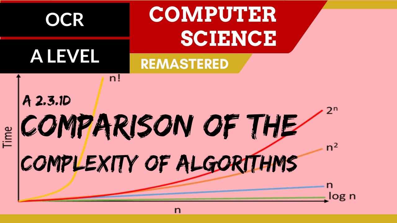
161. OCR A Level (H446) SLR26 - 2.3 Comparison of the complexity of algorithms

EDB1 IMD UFRN (2020.6): Problema de Ordenação
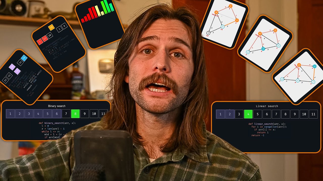
3 Types of Algorithms Every Programmer Needs to Know

Data Structures & Algorithms Roadmap - What You NEED To Learn
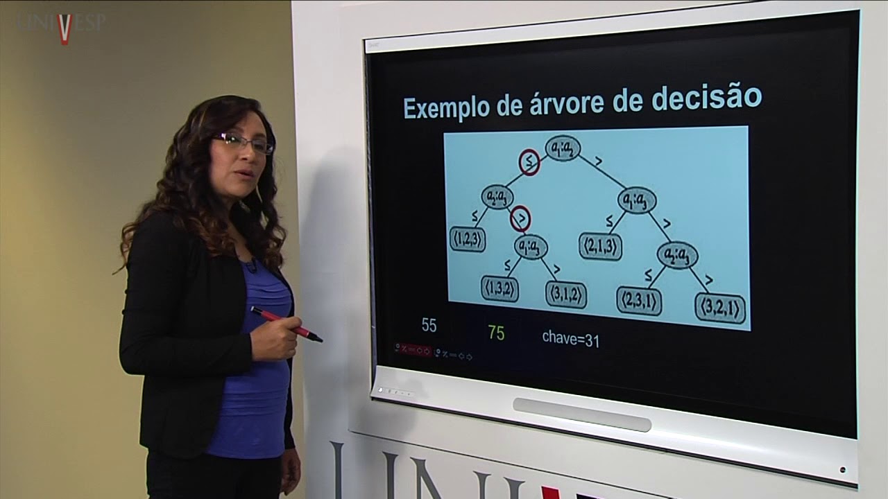
Projeto e Análise de Algoritmos - Aula 09 - Limite inferior para o problema de ordenação

Learn Searching and Sorting Algorithm in Data Structure With Sample Interview Question
5.0 / 5 (0 votes)
